CS331 - Neural Computing
Artificial intelligence is any technique that makes computers act intelligently. Machine learning is a subset of AI in which computers use statistical methods in order to learn. Neural computing is a subset of machine learning which uses brain-inspired neural networks to learn. An example of ML which is not neural computing is Support Vector Machine (SVM) which uses statistical methods which are not brain-inspired. Deep learning is a subset of neural computing which uses deep neural networks with many layers.
Learning paradigms
There are three main paradigms
- Supervised learning uses labelled data to train a model
- Unsupervised learning uses unlabelled data to train a model with no guidance
- Reinforcement learning uses no predefined data. The model learns how to make decisions based on feedback
Supervised learning can be used for classification, such as email filtering or regression. Unsupervised learning can be used for clustering or association.
Semi-supervised learning (SSL) uses a small amount of labelled data and large amounts of unlabelled data.
Inductive learning trains the model on a labelled dataset to learn a general rule that can be applied to make predictions on new, unseen data. Self-learning is a type of induction learning where the model is trained on labelled data, produces predicted pseudo-labels and adds the most confident predictions to the labelled set until all data is labelled.
Transductive learning makes predictions about unlabelled data in the training set given a set of labelled and unlabelled data. Unlike inductive learning the model is trained on the entire dataset, not just the labelled data.
Transfer learning
Transfer learning is a deep learning approach in which a model that has been trained for one task is used as a starting point for a model that performs a similar task. With transfer learning, a pre-existing neural network can be modified slightly to be retrained on a new set of images. Fine-tuning a network with transfer learning is much faster than training a network from scratch.
Transfer learning is commonly used for image and speech recognition. It enables models to be trained with less labelled data by reusing models that have been pre-trained on large data. It can reduce training time and computing resources as weights are not learned from scratch and it can take advantage of good existing model architectures developed by the deep learning research community.
Biological neurons
The central nervous system controls most functions of the body. It consists of the brain and spinal cord. The brain contains billions of neurons. The neuron is the fundamental unit of the nervous system. It is also known as a nerve cell or neural processing unit.
There are several basic elements of a biological neuron
- Dendrite - receives signal from other neurons
- Soma - processes the information, contains DNA
- Axon hillock - controls the firing of the neuron
- Axon - transmits information to other neurons or muscles, the larger the diameter, the faster it transmits information, myelinated axons transmit faster
- Synapse - connect to other neurons
There are three classes of neuron
- Sensory neuron - located in receptors, tell the brain what is happening outside of the body
- Motor neuron - location in the CNS, allow the brain to control muscle movement
- Relay neuron - allow sensory neurons and motor neurons to communicate
The cell membrane is a double layer of lipids and proteins that separates the content of the cell from the external environment. Potassium ions are found inside the cell membrane and sodium ions are found outside. A membrane potential is the difference in electric potential between the inside and outside of the cell membrane. The membrane potential is caused by the unequal distribution of ions.
The neuron is at rest when it is not sending a signal. A resting potential is the difference in voltage across the membrane when a neuron is at rest. It is approximately -70mV. There are two channels in the membrane. Leaky channels are always open, allowing the free passage of sodium and potassium ions across the membrane. Voltage-gated channels are only open at certain voltages and are often closed at resting potential. The resting potential is negative because there is a higher concentration of potassium ions inside the cell meaning they leave through the leaky channels easily. There is also a sodium-potassium pump that uses energy to move three sodium ions out of the neuron for every two potassium ions it puts in.
The action potential is the rapid change in voltage across the membrane when a neuron fires. An action potential is generated when a stimulus changes the membrane potential to above -55mV.
A neuron is polarised if the outside of the membrane is positive and the inside of the membrane is negative. Hyper-polarisation occurs if the membrane becomes more negative then it is at resting potential. A neuron is depolarised if the membrane potential is more positive than it is at the resting potential.
A synapse is a junction between one nerve cell and another. Most synapses are chemical. the action potential is transmitted from the axon terminal to the target dendrites by chemical neurotransmitters. There are excitatory and inhibitory neurotransmitters which stimulate and inhibit cells respectively.
There are four types of synaptic connections
- Axodendritic - axon terminal links to a dendrite
- Axosomatic - axon terminal links to the soma
- Axoaxonal - axon terminal links to the axon
- Dendrodendritic - dendrite links to dendrite
The key components of neural signal processing are
- Signals from neurons are collected by the dendrites
- The soma aggregates the incoming signals
- When sufficient input is received, the neuron generates an action potential
- The action potential is transmitted along the axon to other neurons or to structures outside the nervous system
- If sufficient input is not received, the input will decay and no action potential is generated
- Timing is important - input signals must arrive together, strong inputs will generate more action potentials per unit time
Artificial neural networks
- The first artificial neuron was the MP neuron. The neuron only had 0 and 1 as input and output and had no ability to learn
- The perceptron model was developed for a single-layer neural net which showed an ability to learn but still only output 0 or 1
- ADALINE is an improved perceptron, MADALINE uses multiple layers
- MLP invented, shows perceptrons could not learn the XOR function, leads to AI winter
- Hopfield discovered Hopfield networks, a special form of recurrent neural networks
- The backpropagation algorithm is used to address the XOR learning problem for MLP
- LeNet was the first convolutional neural network (CNN)
- Long short-term memory (LSTM) developed, overcomes the problem of recurrent neural networks forgetting information through layers
The basic structure of an artificial neural network (ANN) consists of an input layer, some number of hidden layers and an output layer. A neural network must have one input and one output layer but can have 0 or more hidden layers. An $N$-layer neural network does not include the input layer in $N$.
A single layer neural network consists of only an input and output layer. A shallow neural network has one or two hidden layers. A deep neural network has three or more hidden layers.
A feedforward neural network is an ANN in which information moves only forwards. There are no cycles or loops in the network.
A convolutional neural network (CNN) uses a series of feature maps to classify input.
Recurrent neural networks (RNN) are feedback neural networks. Information can move both forwards and backwards. RNNs are good for processing temporal sequence data.
MP Neuron
The MP Neuron was the first computational model of a biological neuron. It is also known as a linear threshold gate model. It works similarly to an actual neuron and takes some number of inputs and if their combined signal exceeds a threshold then it produces an output. The diagram for the MP Neuron is
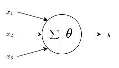
where $\sum$ represents the sum of the input values and $\theta$ represents the threshold.
In this model, the inputs correspond to biological dendrites, the node to the soma and the output to the axon terminal. Unlike synapses in a biological neuron, an MP Neuron does not give different weights to different inputs.
All inputs and outputs are binary. Each input is either excitatory or inhibitory. If any inhibitory input is 1 then the output will be 0 regardless of other inputs. The Rojas diagram for an MP Neuron can be used to represent excitatory and inhibitory inputs
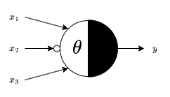
where $\theta$ is the threshold and $x_2$ is an inhibitory input so it has a small circle at the end of the arrow.
The output of MP Neurons can be expressed using vectors. Let $\bm{1} = \begin{bmatrix}1 & 1 & \cdots & 1\end{bmatrix}$ and $\bm{x} = \begin{bmatrix} x_1\\x_2\\\vdots\\x_n\end{bmatrix}$. The sum of the inputs can therefore be expressed as the dot product of these vectors, $z = \bm{1} \cdot \bm{x}$. The threshold can be expressed using a Heaviside function $H_\theta(z) = \begin{cases}1,\quad x \geq \theta\\0,\quad z<\theta\end{cases}$. Therefore, the vector form of the output of the MP Neuron is given by $y = H_\theta(\bm{1} \cdot \bm{x})$.
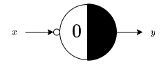
Logic gates can be emulated using MP Neurons. An MP Neuron for the NOT gate has $\theta = 0$ and an inhibitory input. The Rojas diagram for this neuron is
A 2-input AND gate is emulated using a neuron with $\theta = 2$. An $n$-input AND gate is emulated by $\theta = n$. An OR gate is emulated with $\theta = 1$ for any number of inputs.
There are several limitations of the MP Neuron
- Inputs and outputs are limited to binary values only
- All inputs are equally weighted
- The threshold $\theta$ needs to be set manually
Single layer perceptron
The perceptron extends the MP neuron. It can take real numbers as input and each input is weighted. A perceptron is a single-layer neuron and a binary classifier.
A perceptron takes the weighted sum of the input, adds bias and then applies a threshold to determine the binary output.
Perceptron learning works by updating the weights until all nodes are correctly classified.
The vector form of a perceptron consists of a weight vector, $\bm{w}$, and input vector, $\bm{x}$. The weighted sum of inputs including the bias, $b$, is given by $\bm{w} \cdot \bm{x} + b$. The output of the perceptron is given by $y = H(\bm{w} \cdot \bm{x} + b)$. The bias can alternatively be included at the end of the weight vector by adding 1 to the end of the input vector.
The dot product can be used to find the angle between vectors. If the dot product is 0 then the vectors are at right angles, if it is less than 0 then the angle is obtuse and more than 0 is acute.
A node is correctly classified if the angle between it and the weight vector is acute. If a node is misclassified then it can be added to or subtracted from the weight vector. A learning rate hyperparameter which determines the step size at each iteration of training can be used to improve accuracy at the cost of speed.
Multi-layer perceptron
XOR cannot be represented with a single layer perceptron because it is not linearly separable. This can be resolved by either changing the threshold function or using multiple perceptrons. $a \oplus b = (a \cup b) \cap \neg(a \cap b)$ and $\cap, \cup$ and $\neg$ can be emulated with a perceptron so multiple perceptrons can be used to emulate the XOR function. More generally, multiple perceptrons can be combined to recognise more complex subsets of data.
Activation functions
An activation function is a mathematical function attached to each neuron which decides if it should be activated. It adds non-linearity to neural networks and normalises the output of each neuron. The Heaviside function is a simple activation function.
Linear activation functions allow for multiple output values but don't allow for complex relationships with the input.
The sigmoid function, $\sigma(x) = \frac{1}{1+e^{-x}}$ is similar to a step function with a smooth gradient. This allows for more confident classification of inputs and output values are normalised between 0 and 1. The sigmoid function has a vanishing gradient and for very large or small inputs there is almost no change to prediction which inhibits the ability to learn. Another problem is that the sigmoid function is not zero-centred and computationally expensive. The first derivative of the sigmoid function is given by $\sigma'(x) = \sigma(x) \cdot (1-\sigma(x))$.
The $\tanh$ function is given by $$ \frac{e^x-e^{-x}}{e^x+e^{-x}} $$ Unlike the sigmoid function, $\tanh$ is zero centred and output is normalised between -1 and 1. Like the sigmoid function, it still has the vanishing gradient problem and is computationally expensive. This is because the functions are related, $\tanh(x) = 2\cdot\sigma(2x) - 1$. The first derivative of $\tanh$ is given by $\tanh'(x) = 1-\tanh^2(x)$.
The Rectified Linear Unit (ReLU) function is given by $$ \operatorname{ReLU}(x) = \max(0, x) = \begin{cases}x, & x \geq 0\\0, & x < 0\end{cases} $$ The ReLU function is easy to compute and has no vanishing gradient for positive values. The dying ReLU problem occurs when a neuron receives negative input and then only outputs 0. It is also not a zero-centred function.
The leaky ReLU function resolves the dying ReLU problem and is given by $$ \operatorname{LReLU}(x) = \max(\alpha x, x) = \begin{cases}x, & x \geq 0\\\alpha x, & x < 0\end{cases} $$ for some $\alpha$.
Parametric ReLU (PReLU) is a variation of LReLU which makes $\alpha$ a learnable parameter. This is more computationally expensive.
The Exponential Linear Unit (ELU) function is given by $$ \operatorname{ELU}(x) = \begin{cases}x, & x \geq 0\\\alpha(e^x-1), & x < 0\end{cases} $$ This is smoother at $x=0$ than LReLU, does not have the dying ReLU problem and has no vanishing gradient problem for $x \geq 0$. There is still a vanishing gradient problem for $x \leq 0$ and it is more computationally expensive than ReLU and LReLU.
The softmax function is a generalisation of the sigmoid function. It takes as input a vector $z$ of $N$ real values and normalises it into a probability distribution consisting of $N$ probabilities proportional to the exponentials of the input values. $$ y_i = \frac{e^{z_i}}{\sum_{j=1}^Ne^{z_j}} $$ Because this is a probability distribution, $\sum_{i=1}^N y_i = 1$.
The exponential function is needed to account for negative input values as probabilities have to be positive. When $N=2$, the softmax function reduces to the sigmoid function.
The maxout function is a generalisation of ReLU. $$ y = M_k(x) = \max \{w_1x+b_1, w_2x+b_2,\cdots, w_kx+b_k \} $$ where $k$ is the number of affine feature maps, $x$ is the input and $w_i$ and $b_i$ are learnable weights. A single maxout unit can approximately learn any convex function. Two maxout units can approximately learn any continuous function. The maxout function increases the number of hidden neurons and training parameters meaning it is very computationally expensive.
Forward propagation
Forward propagation feeds data forwards through the network. Each hidden layer receives data from the previous layer, processes it and passes it to the next.
The output of a neural network can be computed using either element-wise or by using matrices.
The output at each layer is given by $\bm{z} = f(\bm{w} \cdot \bm{x} + \bm{b})$ where $\bm{w}, \bm{x}$ and $\bm{b}$ are the weights, input and bias for each neuron respectively and $f$ is the activation function.
Vectorisation is an optimisation technique that converts an element-wise operation to one that uses matrices or vectors. Modern CPUs have direct support for vector operations and these are much faster than the element-wise equivalent.
Loss functions and regularisation
A loss function measures the difference between the value predicted by a neural network, $\hat{y}$ and the target value, $y$.
A good loss function
- Is minimised when the predicted value is equal to the target
- Increases when the difference between predicted and target increases
- Is globally continuous and differentiable
- Is convex
The loss function is for a single training input/output pair. The cost function is the average loss function over the entire training set.
There are two groups of loss functions, regression and classification. Regression functions predict continuous, numeric values. Classification functions predict categorical values.
The L1 loss function is given by $L(\hat{y}, y) = |\hat{y} - y|$. This function is intuitive and fast but not differentiable at $\hat{y} = y$ and is less sensitive to outliers. Its cost function is the Mean Absolute Error (MAE) which is given by $\frac{1}{n}\sum_{i=1}^n|\hat{y}_i - y_i|$.
The L2 loss function is given by $L(\hat{y}, y) = (\hat{y}-y)^2$. This function is sensitive to outliers and penalises large errors more strongly but outliers will result in much larger errors. Its cost function is the Mean Squared Error (MSE) which is given by $\frac{1}{n}\sum_{i=1}^n(\hat{y}_i - y_i)^2$.
[missing vector norm stuff]
The L0 norm of a vector is the number of non-zero entries it contains. This is useful for finding the sparsest solution to a set of equations. The L0 norm can be used to limit the number of features to learn from training data which prevents over and underfitting.
Regularisation discourages learning more complex features by applying a penalty to the input parameters with larger weights to avoid the risk of overfitting. Regularisation constrains weights towards 0.
Regularisation using the L0 norm is NP-hard, so L1 and L2 are used instead as these are easier to compute. L1 regularisation is also known as lasso regularisation. L2 regularisation is also known as ridge regularisation.
The log or cross entropy loss function measures the accuracy of a classification model. Log loss compares predicted output $\hat{y}$ with true class $y$ and penalises the probability logarithmically based on how far it diverges from the true class. The log loss function is given by $$ L(\hat{y}, y) = -y\log \hat{y}-(1-y)\log(1-\hat{y}) $$ The $N$-class log loss function is given by $$ L = -\sum_{i=1}^N y_i\log\hat{y}_i $$ with $\sum y_i = 1$ and $\sum \hat{y}_i = 1$.
Backpropagation
Gradient descent is an iterative algorithm that finds a minimal value, $v$, of a function, $f$, given an initial point, $x_0$ such that $$ v = \min_x f(x) $$ Gradient descent works by repeatedly finding $$ x_{t+1} = x_t - \alpha\cdot\nabla f(x_t) $$ where $\alpha$ is a configurable hyperparameter that controls how much the weights are adjusted with respect to the loss gradient.
For example, let $f(x) = x^2 - 2x$, $x_0 = 4$ and $\alpha = 0.4$. The minimum value is given by $$ \begin{aligned} x_1 &= x_0 - 0.4 \times f'(4) = 1.6 \\ x_2 &= x_1 - 0.4 \times f'(1.6) = 1.12\\ x_3 &= 1.02 \\ &\cdots \\ x_n &= 1 \end{aligned} $$ so the minimum value is given by $f(1) = -1$.
For a neural network, gradient descent is used to minimise the loss function. Backpropagation is an effective way of training a neural network by minimising the cost function by adjusting the weights and biases of the network.
The steps to train a neural network are as follows
- Initialise weights and bias at random
- Use forward propagation to compute expected output $\hat{y}$
- Use loss function to measure the error between $\hat{y}$ and target $y$
- Use backpropagation to minimise the loss fiction by adjusting the weights and bias through gradient descent
- Repeat 2-4 until loss function is minimised
Hopfield network
Hopfield networks (HNs) are based on fixed-point iteration, in which an initial guess converges towards the nearest stable fixed point.
Associative learning involves forming associations between items. A HN uses associate memory to associate an input to its most similar memorised output.
Associative memory, also known as Content Addressable Memory (CAM), is the ability to retrieve an item by knowing part of its content.
An $n \times n$ pattern can be represented as a $n^2 \times 1$ vector $\vec{x}$. Each element $x_i$ denotes a state of a neuron $i$. For a discrete HN, each state takes either
- Bipolar values - 1 firing, -1 non-firing
- Binary values - 1 firing, 0 non-firing
The HN is a special form of RNN. It is a single layer, fully connected auto-associative network. Neurons act as both input and output with a binary threshold. HNs are widely used for pattern recognition.
The graph of a HN is a complete graph $G = (V, E)$ where a node $i \in V$ is a perceptron with a state, a pair $(i, j) \in E$ links a pair of nodes with a weight $W_{ij}$. Edges are traversed in both directions and there are no self loops.
The Hebbian learning rules state that
- Neurons that fire together wire together
- Neurons that fire out of sync fail to link
This means simultaneous activation of neurons leads to increased synaptic strength between them.
The weight matrix for a single memorised pattern is given by $$ W = \vec{x} \cdot \vec{x}^T - I $$ $\vec{x} \cdot \vec{x}^T$ is called the rank-one matrix. Subtracting the identity matrix removes the self-loops.
The weight matrix for multiple patterns is given by the average of their weight matrices.
A neuron in a HN has a stable state if the following holds $$ \vec{s}(t+1) = F(W \cdot \vec{s}(t)) $$ where $\vec{s}(t)$ is the state of the HN at time $t$.
For bipolar HN, the activation function is $F = \begin{cases}1 & x \geq0 \\ -1 & x <0 \end{cases}$.
For a memorised pattern $\vec{x}$ to be a fixed-point for the HN it has to satisfy $\vec{x} = F(W \cdot \vec{x})$. A single memorised pattern is always stable.
The energy of a HN is the capacity of the network to evolve. The network will evolve until it arrives at a local minimum in the energy contour. The energy of a HN is given by $$ E = -\sum_{i=1}^n\sum_{j>i}s_i W_{ij}s_j $$ where $s_i$ and $s_j$ are neurons with common weight $W_{ij}$.
The matrix form is given by $$ E = -\frac{1}{2}\vec{s}^TW\vec{s} $$
The energy decreases each time a neuron state changes so $E$ is a decreasing function.
Recurrent neural networks
A Recurrent Neural Network (RNN) is a type of neural network that processes sequential or time series data. RNNs can use their internal state to process variable length sequences of inputs.
Named Entity Recognition (NER) is an information extraction task that locates and classifies named entities in text into pre-defined categories such as names, locations or dates. This is more suited to RNNs than feedforward networks as it makes use of surrounding words for context.
Unlike in a feedforward network, the order of input is important for an RNN.
Elman networks feedback from the internal state output (before weighting the output) to the input. There are weights associated with the input, output and the hidden layer. In Jordan networks the network output (after weighting the output) feeds back to the input.
The output of an Elman RNN is given by $y_t = \sigma(W_o \cdot a_t)$ with $a_t = \tanh(W_i \cdot x_t + W_h \cdot a_{t-1})$ where $W_i$, $W_h$ and $W_o$ are the input, hidden and output weights respectively.
The output of a Jordan RNN is given by $y_t = \sigma(W_o \cdot a_t + b_o)$ with $a_t = \tanh(W_i \cdot x_t + W_h \cdot y_{t-1})$.
Simple RNNs only have a single unidirectional hidden layer. There are several variations
- Deep Recurrent Neural Networks (DRNN)
- Bidirectional Recurrent Neural Networks (BRNN)
- Long Short-Term Memory (LSTM)
- Gated Recurrent Units (GRU)
An RNN can be deep with respect to time and space. A deep RNN is constructed by stacking layers of RNN together. The hidden state information is passed to the next time step of the current layer and the current time step of the next layer.
There are two ways of introducing depth to RNNs
- expanding looping operations into multiple hidden units
- increasing computational depth of a hidden unit
Bidirectional RNNs allow RNNs to have both backward and forward information about the input at every time step.
Simple RNNs are susceptible to the vanishing and exploding gradient problems. For example, a weight of 0.9 after 100 iterations becomes $0.9^{100} = 0.000017\dots$ and a weight of 1.1 becomes $1.1^{100} = 13780.61\dots$. These demonstrate the vanishing and exploding gradient problems respectively. These problems make it difficult for an RNN to capture long term dependencies.
The exploding gradient problem can be reduced by using gradient clipping, where the gradient limited to a threshold value. Vanishing gradient can be reduced using LSTM.
LSTM is a type of RNN which uses three types of gates to control the flow of information passed through the memory cell. The three gates are
- Input gate (i) which controls if data can enter the memory
- Output gate (o) which controls if data can be output from the memory
- Forget gate (f) which controls if all previous data in the memory can be forgotten
$(i_t, o_t, f_t)$ denotes the state of the different gates at time step $t$. When $i_t$ is 1, input is allowed, when it is 0 input is not allowed. $o_t$ allows output when 1, disallow when 0. $f_t$ forgets when 0, remembers when 1.
The equations for LSTM are as follows $$ \begin{aligned} c_t &\leftarrow f_t * c_{t-1} + i_t * a_t\\ a_t &\leftarrow \tanh\left(W \begin{bmatrix} \frac{h_{t-1}}{x_t} \end{bmatrix}\right)\\ h_t &\leftarrow o_t * \tanh(c_t)\\ \begin{bmatrix} f_t \\ i_t \\ o_t \end{bmatrix} &\leftarrow \sigma\left(\begin{bmatrix} W_f \\ W_i \\ W_o \end{bmatrix}\begin{bmatrix} \frac{h_{t-1}}{x_t} \end{bmatrix}\right) \end{aligned} $$ where $c_t$ is the memory state, $a_t$ is the activation value and $h_t$ is the hidden state.
Different RNNs are used for different length inputs and outputs
- One to one
- One to many
- Many to one, can be used for sentiment analysis
- Many to many, can be used for named entity recognition or machine translation
Graph mining
There are several ways of representing graphs
- Adjacency matrix - $(i,j)$ th element is the weight of the edge between $i$ and $j$, requires $O(|V|^2)$ space, ideal for dense graphs, connectivity can be determined in $O(1)$ time, powers of matrix give the number of paths of that length between two nodes
- Laplacian matrix - Given by the degree matrix minus the adjacency matrix, the number of spanning trees in a connected graph is the determinant of any cofactor of the Laplacian matrix, ideal for dense graphs
- Adjacency list - Graph represented as an array of linked lists containing the out-neighbours of each node, requires $O(|E| + |V|)$ space, more efficient for sparse matrices
- Compressed Sparse Row (CSR) - Represents a matrix as a row offset, column index and value
- Coordinate list - Represents a matrix as row index, column index and value
PageRank
PageRank is a ranking algorithm that rates the importance of a webpage recursively based on graph structures. A webpage is considered important if it is pointed to by many important webpages.
A simplified version of PageRank is given by $$ PR(v) = \sum_{x \in I(v)} \frac{PR(x)}{|O(x)|} $$ where $I(x)$ and $O(x)$ are the incoming and outgoing edges of node $x$ respectively.
Simplified PageRank does not work if a node does not have in-neighbours or the graph has cycles.
The Classic PageRank model adds a damping factor $0 \leq c \leq 1$. The algorithm keeps walking with probability $c$ but jumps to another node with probability $1-c$. This prevents the problems with the simplified PageRank algorithm. The Classic PageRank model is given by $$ PR(v) = c\sum_{x \in I(v)}\frac{PR(x)}{|O(x)|} + (1-c)\frac{1}{|V|} $$
The matrix form of PageRank is given by $$ \bm{p} = c\bm{W}\bm{p} + \frac{1-c}{|V|}\bm{1} $$ where $\bm{p}$ is the PageRank vector $\bm{p} = \left[PR(1), \cdots, PR(n)\right]^T$, $\bm{W}$ is a transition matrix and $\bm{1}$ is a vector of 1s.
The transition matrix is given by $$ W_{i,j} = \begin{cases} \frac{1}{|O(j)|} & \text{if } \exists (j, i) \in E \\ 0 & \text{otherwise} \end{cases} $$ The transition matrix is the column normalised adjacency matrix of the graph. This can be denoted $\bm{W} = \bm{A}^T(\bm{D}^{-1})$ where $D$ is the diagonal out-degree matrix.
$\bm{W}$ is column-stochastic because each column sums to 1 and each element is between 0 and 1. $\bm{W}$ describes the transition of a Markov Chain.
The PageRank vector $\bm{p}$ is defined recursively. There are three methods to calculate the PageRank vector
- Fixed-point iteration
- Matrix inversion
- Dominant eigenvector
For fixed-point iteration, let $\bm{p}_ 0 = \frac{1}{|V|}\bm{1}$ and $\bm{p}_ k = c\bm{W}\bm{p}_ {k-1} + \frac{1-c}{|V|}\bm{1}$. $\bm{p_ k} \rightarrow \bm{p}$ as $k \rightarrow \infty$. The number of iterations needed to achieve a desired accuracy $\epsilon$ is given by $k \geq \lceil\log_c(\epsilon/2)\rceil + 1$. The time and space complexity of each iteration is $O(|E| + |V|)$.
Another method is matrix inversion. The PageRank equation can be rearranged to collect $\bm{p}$ on one side $$ \begin{aligned} \bm{p} &= c\bm{W}\bm{p} + \frac{1-c}{|V|}\bm{1}\\ (\bm{I} - c\bm{W})\bm{p} &= \frac{1-c}{|V|}\bm{1}\\ \bm{p} &= \frac{1-c}{|V|}\left(\bm{I} - c\bm{W}\right)^{-1}\bm{1} \end{aligned} $$ This is the closed form of PageRank. The inverse of $\bm{I} - c\bm{W}$ always exists but is expensive to find and very dense. The time and space complexities are $O(|V|^3)$ and $O(|V|^2)$ respectively. This is much slower and uses more space than fixed-point iteration but provides an exact solution.
Another method is using the dominant eigenvector. $||\bm{p}||_1 = 1$ can be rearranged to give $\bm{1}^T\bm{p} = 1$. Multiplying the original equation by 1 gives $$ \begin{aligned} \bm{p} &= c\bm{W}\bm{p} + \frac{1-c}{|V|}\bm{1} \cdot 1 \\ \bm{p} &= c\bm{W}\bm{p} + \frac{1-c}{|V|}\bm{1} \cdot \bm{1}^T\bm{p} \\ \bm{p} &= \left(c\bm{W} + \frac{1-c}{|V|}\bm{1} \cdot \bm{1}^T\right)\bm{p} \end{aligned} $$ The Google matrix $G$ is given by $$ \bm{G}= c\bm{W} + \frac{1-c}{|V|}\bm{1} \cdot \bm{1}^T $$ so the PageRank equation can be expressed as $\bm{p} = \bm{G}\bm{p}$.
HITS
Hyperlink-Induced Topic Search (HITS) is a PageRank-like ranking algorithm that measures the importance of webpages based on authority and hub scores of each webpage. A good webpage should link to other good webpages and be linked by other good webpages.
The authority score $a(x)$ of a node $x$ is given by the sum of the scaled hub scores of its neighbours. The hub score, $h(x)$, is given by the sum of the scaled authority scores of the out-neighbours of $x$.
HITS can be evaluated using three methods
- Iterative
- Dominant eigenvector
- Singular Value Decomposition (SVD)
Graph-based similarity search
Graph-based Jaccard similarity of two nodes $a$ and $b$ is given by $$ \operatorname{sim}(a, b) = \frac{|I(a) \cap I(b)|}{|I(a) \cup I(b)|} $$ where $I(x)$ is the set of incoming neighbours.
Jaccard graph search does not consider the number of common neighbours and does not consider greater than one-hop similarity.
SimRank considers multi-hop neighbours. The SimRank similarity of two nodes $a$ and $b$ is given by $$ s(a,b) = \begin{cases} 0 & \text{if } I(a) = \emptyset \text{ or } I(b) = \emptyset\\ \frac{C}{|I(a)||I(b)|}\sum_{x \in I(a)}\sum_{y \in I(b)}s(x, y) & \text{if } a \neq b\\ 1 & \text{if } a = b \end{cases} $$ where $C$ is a damping factor.
The similarity of all pairs of nodes in a graph is given by $$ \bm{S}_ i = \max\{C \cdot \bm{Q}^T\bm{S}_ {i-1}\bm{Q}, \bm{I}\} $$ where $Q$ is the column-normalised adjacency matrix and $\bm{S}_i$ is the matrix of SimRank values and $\bm{S}_0 = \bm{I}$. The minimum number of iterations needed to achieve accuracy $\epsilon$ is $k\geq \lceil\log_c\epsilon\rceil$.
Dimensionality reduction for time series
Dimensionality reduction reduces the dimension of a data set. This can avoid overfitting, eliminate noise and reduce the amount of space required.
There are three dimensionality reduction techniques
- Piecewise Aggregate Approximation (PAA) - Split the time series into equally sized segments and use the average value for each segment, takes $O(n)$ time for a time series of length $n$
- Piecewise Linear Approximation (PLA) - Approximates each segment of a time series using the best-fit coefficients of the equation of a line
- Adaptive Piecewise Constant Approximation (APCA) - Adaptive PAA, allows for variable length segments