CS262 - Logic and Verification
Propositional logic is a formal system for reasoning about propositions. A proposition may also be called a statement or formula. Atomic propositions can not be split. Atomic propositions can be joined using logical connectives to form new propositions. Common connectives include $\neg$, $\wedge$, $\vee$ and $\rightarrow$. Binary connective can generally be denoted using $\circ$. For example, $\circ = \{\wedge, \vee, \rightarrow, ...\}$.
Atomic formulae include propositional variables and $\top$ or $\bot$. If $X$ is a formula so is $\neg X$. If $X$ and $Y$ are formulae then so is $X \circ Y$.
A parse tree can be constructed for any propositional formula. An atomic formula $X$ has a single node labelled $X$. The subtree for $\neg X$ has a node labelled $\neg$ with the subtree $X$ as a child. The parse tree for $X \circ Y$ has a node labelled $\circ$ as the root and the parse trees for $X$ and $Y$ as left and right subtrees respectively.
In propositional logic, formulae can have one of two possible values, T or F. A truth table lists each possible combination of truth values for the variables of a Boolean function.
A valuation is a mapping $v$ from the set of propositional formula to the set of truth values satisfying the following conditions:
- $v(T) = T$, $v(F) = F$
- $v(\neg X) = \neg v(X)$
- $v(X \circ Y) = v(X) \circ v(Y)$
The truth table of a formula lists all possible valuations.
A formula that evaluates to T under all valuations is a tautology. A formula that evaluated to F under all valuations is a contradiction. A formula that evaluates to T for some valuation is called satisfiable.
A formula $X$ is a consequence of a set $S$ of formulae, denoted $S \vDash X$, provided $X$ maps to T under every valuation that maps every member of $S$ to T. $X$ is a tautology if and only if $\emptyset \vDash X$, which is written as $\vDash X$. More simply, $S$ is the set of formulae which need to be true for $X$ to be true.
Formulae representing the same truth function are called logically equivalent. $p \rightarrow q = \neg p \vee q$.
Normal forms
A set of connectives is said to be complete if we can represent every truth function $\{T,F\}^n \rightarrow \{T, F\}$ using only these connectives.
Consider a function $f$ on variables $x_1, ..., x_n$. For the values $v_i$ where $f(v_1, ..., v_n) = T$, if $v_i$ is T then replace it with $x_i$ or $\neg x_i$ if $v_i$ is F and take the conjunction. Then take the disjunction of these conjunctions. This shows that $\{\wedge, \vee, \neg\}$ is complete as any formula can be expressed using only these connectives. The resulting formula is said to be in disjunctive normal form (DNF). The DNF of a function of not unique.
A literal is a variable, its negation, $\bot$ or $\top$.
DNF is the disjunction of conjunctions of literals.
Conjunctive normal form (CNF) is the conjunction of disjunctions of literals.
Every Boolean function has a CNF and DNF.
Let $X_1, X_2, ..., X_n$ be a sequence of propositional formulas.
A generalised disjunction is written as $[X_1,X_2,...,X_n] = X_1 \vee X_2 \vee ... \vee X_n$.
A generalised conjunction is written as $\left<X_1, X_2, ..., X_n\right> = X_1 \wedge X_2 \wedge ... \wedge X_n$.
If $X_1, ... X_n$ are literals then $[X_1, ...]$ is a clause and $\left< X_1, ...\right>$ is a dual clause.
$v([]) = F$ and $v(\left<\right>) = T$. These are the neutral element of disjunction and conjunction respectively.
$\alpha$ and $\beta$ formulae
All propositional formulae of the forms $X \circ Y$ and $\neg(X \circ Y)$ are grouped into two categories, those that act conjunctively and those that act disjunctively.
The below tables can be derived from the following definitions:
- $\alpha = \alpha_1 \wedge \alpha_2$
- $\beta = \beta_1 \vee \beta_2$
Conjunctive
| $\alpha$ | $\alpha_1$ | $\alpha_2$ |
|---|---|---|
| $X \wedge Y$ | $X$ | $Y$ |
| $\neg(X \vee Y)$ | $\neg X$ | $\neg Y$ |
| $\neg(X \rightarrow Y)$ | $X$ | $\neg Y$ |
| $\neg(X \leftarrow Y)$ | $\neg X$ | $Y$ |
| $\neg(X \uparrow Y)$ | $X$ | $Y$ |
| $X \downarrow Y$ | $\neg X$ | $\neg Y$ |
| $X \not\rightarrow Y$ | $X$ | $\neg Y$ |
| $X \not\leftarrow Y$ | $\neg X$ | $Y$ |
Disjunctive
| $\beta$ | $\beta_1$ | $\beta_2$ |
|---|---|---|
| $\neg(X \wedge Y)$ | $\neg X$ | $\neg Y$ |
| $X \vee Y$ | $X$ | $Y$ |
| $X \rightarrow Y$ | $\neg X$ | $Y$ |
| $X \leftarrow Y$ | $X$ | $\neg Y$ |
| $X \uparrow Y$ | $\neg X$ | $\neg Y$ |
| $\neg(X \downarrow Y)$ | $X$ | $Y$ |
| $\neg(X \not\rightarrow Y)$ | $\neg X$ | $Y$ |
| $\neg(X \not\leftarrow Y)$ | $X$ | $\neg Y$ |
For every $\alpha$- and $\beta$-formula valuation
- $v(\alpha) = v(\alpha_1) \wedge v(\alpha_2)$
- $v(\beta) = v(\beta_1) \vee v(\beta_2)$
CNF algorithm
Given any propositional formula, find $\left<\left[X\right]\right>$, which will give a conjunction of disjunctions of the form $\left<D_1, ..., D_n\right>$. Select one of these disjunctions which is not a disjunction of literals, and denote it $D_i$. Select a non-literal $N$ from $D_i$.
- If $N = \neg \top$ then replace $N$ with $\bot$
- If $N = \neg \bot$ then replace $N$ with $\top$
- If $N = \neg \neg Z$ then replace $N$ with $Z$
- If $N$ is a $\beta$-formula then replace $N$ with $\beta_1 \vee \beta_2$ (this is called $\beta$-expansion)
- If $N$ is a $\alpha$-formula then replace $D_i$ with two disjunctions, one in which $N$ is replaced with $\alpha_1$ and one in which $N$ is replaced by $\alpha_2$.
Example
$\neg(p\wedge \neg \bot) \vee \neg(\top \uparrow q)$
- Take conjunction of disjunction: $\left<\left[\neg(p\wedge \neg \bot) \vee \neg(\top \uparrow q)\right]\right>$
- Apply $\beta$ expansion: $\left<\left[\neg(p\wedge \neg \bot), \neg(\top \uparrow q)\right]\right>$
- Apply $\beta$ expansion: $\left<\left[\neg p, \neg \neg \bot, \neg(\top \uparrow q)\right]\right>$
- Apply double negation: $\left<\left[\neg p, \bot, \neg(\top \uparrow q)\right]\right>$
- Apply $\alpha$ expansion: $\left<\left[\neg p, \bot, \top\right], \left[\neg p, \bot, q\right]\right>$
- Formula is now in CNF, stop.
Correctness of the algorithm
The algorithm produces a sequence of logically equivalent formulas.
The proof for $\beta$-expansion is trivial. $\alpha$-expansion can be demonstrated by distributivity: $D_i = [\alpha, X_2, ...,X_k]$ is equivalent to $(\alpha_1 \wedge \alpha_2) \vee (X_2 \vee ... \vee X_k)$ which by distributivity is $(\alpha_1 \vee (X_2 \vee ... \vee X_k)) \wedge (\alpha_2 \vee (X_2 \vee ... \vee X_k))$ which, by associativity, can be written as $\left<\left[\alpha_1, X_2, ..., X_k\right], \left[\alpha_2, X_2, ..., X_k\right]\right>$
The algorithm terminates, regardless of which choices are made during the algorithm.
Consider a rooted tree. A branch is a sequence of nodes starting at the root and finishing at a leaf. A tree is finitely branching if every node has finitely many children. A tree/branch is finite if it has a finite number of nodes.
König's lemma states that a tree that is finitely branching but infinite must have an infinite branch.
The rank, $r$, of a propositional formula is defined as follows
- $r(p) = r(\neg p) = 0$ for variables $p$
- $r(\top) = r(\bot) = 0$
- $r(\neg \top) = r(\neg \bot) = 1$
- $r(\neg \neg Z) = r(Z) + 1$
- $r(\alpha) = r(\alpha_1) + r(\alpha_2) + 1$
- $r(\beta) = r(\beta_1) + r(\beta_2) + 1$
- $r\left(\left[X_1, ..., X_n\right]\right) = \sum^n_{i=1}r(X_1)$
Example
$r((m \rightarrow \neg n) \wedge (\neg \neg o \wedge \neg \bot))$
- $r(m) = r(\neg m) = r(\neg n) = 0$
- $r(\neg \neg o) = r(o) + 1 = 0 + 1 = 1$
- $r(\neg \bot) = 1$
- $r(m \rightarrow \neg n) = r(\neg m) + r(\neg n) + 1 = 0 + 0 + 1 = 1$
- $r(\neg \neg o \wedge \neg \bot) = r(\neg \neg o) + r(\neg \bot) + 1 = 1 + 1 + 1 = 3$
- $r((m \rightarrow \neg n) \wedge (\neg \neg o \wedge \neg \bot)) = r(m \rightarrow \neg n) + r(\neg \neg o \wedge \neg \bot) + 1 = 1 + 3 + 1 = 5$
so the rank of the formula is 5.
A CNF expression is of the form $\left<\left[D_1, ..., D_n\right]\right>$. Each $D_i$ can be assigned a rank. Every step in the CNF algorithm decreases the rank of the disjunction or replaces it with two disjunctions of lower rank (in the case of $\alpha$-expansion). Consider each of the 5 rules of the CNF algorithm:
- Negation of $\top$ and $\bot$ will reduce rank from 1 to 0
- Double negation will reduce rank by 1
- $r(\alpha) = r(\alpha_1) + r(\alpha_2) + 1$, so $r(\alpha_1)$ and $r(\alpha_2)$ are both less than $r(\alpha)$. Therefore the two replacement disjunctions must each have lower rank.
- $r(\beta) = r(\beta_1) + r(\beta_2) + 1$ so the new disjunction has lower rank.
Given the above, an infinite branch is not possible, so the algorithm must terminate by König's theorem.
DNF algorithm
The DNF algorithm works very similarly to CNF. It starts by finding $\left[\left<X\right>\right]$. The first 3 rules are the same, but $\alpha$-expansion replaces a conjunction with $\alpha_1, \alpha_2$ and $\beta$-expansion replaces a conjunction with $\left[\left<..., \beta_1, ...\right>,\left<..., \beta_2, ...\right>\right]$, the opposite to the rules for a CNF.
Example
$\neg(p\wedge \neg \bot) \vee \neg(\top \uparrow q)$
- Take the disjunction of conjunctions: $\left[\left<\neg(p\wedge \neg \bot) \vee \neg(\top \uparrow q)\right>\right]$
- Apply $\beta$-expansion: $\left[\left<\neg(p\wedge \neg \bot)\right>,\left<\neg(\top \uparrow q)\right>\right]$
- Apply $\alpha$-expansion: $\left[\left<\neg(p\wedge \neg \bot)\right>,\left<\top, q\right>\right]$
- Apply $\beta$-expansion: $\left[\left<\neg p\right>, \left<\neg \neg \bot \right>, \left<\top, q\right>\right]$
- Apply double negation: $\left[\left<\neg p\right>, \left<\bot \right>, \left<\top, q\right>\right]$
- Formula is now in DNF, stop
Semantic tableau
There are two proof procedures for propositional logic - semantic tableau and resolution, closely connected to DNF and CNF respectively.
Both are refutation systems - to prove that a formula $X$ is a tautology, it begins with $\neg X$ and finds a contradiction.
Semantic tableau takes the form of a binary tree with nodes labelled with propositional formulae. Each branch can be seen as a conjunction of formulae on that branch and the tree is a disjunctions of all of its branches, hence DNF.
The tableau (tree) can be expanded. Select a branch and a non-literal formula $N$ on the branch
- If $N = \neg\top$ then extend the branch by a node labelled $\bot$ at its end
- If $N = \neg \bot$ then extend the branch by a node labelled $\top$ at its end
- If $N = \neg \neg Z$ then extend the branch by a node labelled $Z$ at its end
- If $N$ is an $\alpha$-formula, extend the branch by two nodes labelled $\alpha_1$, $\alpha_2$ ($\alpha$-expansion) at its end
- If $N$ is a $\beta$-formula, add a left and right child to the final node of the branch, labelled $\beta_1$ and $\beta_2$ ($\beta$-expansion)
Example
$\neg((p \rightarrow (q \rightarrow r)) \rightarrow ((p \vee s) \rightarrow ((q \rightarrow r) \vee s)))$
The following tree shows a partial expansion of the formula:
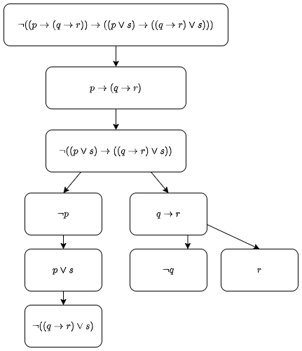
The formula is the root node. This is then $\alpha$-expanded to give two nodes. $p \rightarrow (q \rightarrow r)$ is then $\beta$-expanded to give a $\neg p$ and $q \rightarrow r$ as children at the end of the branch. $q \rightarrow r$ is $\beta$-expanded to give two literal children. $\neg((p \vee s)...)$ is $\alpha$-expanded to the two nodes at the end of the left branch.
A branch of a tableau is closed if both $X$ and $\neg X$ occur on the branch for some formula $X$ or if $\bot$ occurs on the branch. If $x$ and $\neg x$ appear on a branch then the branch is atomically closed. A tableau is (atomically) closed if every branch is (atomically) closed. A tableau proof for $X$ is a closed tableau for $\neg X$. If $X$ has a tableau proof this can be denoted $\vdash_t X$.
Example
$X = (p \wedge (q \rightarrow (r \vee s))) \rightarrow (p \vee q)$
The above is closed because $p$ and $\neg p$ appear on the same branch. As this is the only branch the tableau is closed, meaning $X$ is a tautology.
A tableau is strict is no formula has had an expansion rule applied to it twice on the same branch.
To implement semantic tableau, the tree can be represented as a list of lists (disjunction of conjunctions). The strictness rule allows an expanded formula to be removed from a list. This is the same method as DNF expansion but it stops when a contradiction is found instead of continuing to literals.
The tableau proof system is sound - if $X$ has a tableau proof then $X$ is a tautology. This is proven by the correctness of DNF.
The tableau proof system is complete - if $X$ is a tautology then the strict tableau system will terminate with a proof for it.
Resolution proofs
Resolution proofs are closely linked to CNF expansion. Unlike semantic tableau, resolution proofs don't use a tree, they use $\left<\left[\dots\right],\dots,\left[\dots\right]\right>$ notation.
Like semantic tableau, resolution proof begins with the negation of the expression to prove.
In each step, select a disjunction and a non-literal formula $N$ in it
- If $N = \neg \top$, append a new disjunction where $N$ is replaced by $\bot$
- If $N = \neg \bot$, append a new disjunction where $N$ is replaced by $\top$
- If $N = \neg \neg Z$, append a new disjunction where $N$ is replaced by $Z$.
- If $N$ is an $\alpha$-formula, append two new disjunctions, one in which $N$ is replaced by $\alpha_1$ and another in which it is replaced by $\alpha_2$
- If $N$ is a $\beta$-formula, append a new disjunction where $N$ is replaced by $\beta_1, \beta_2$
A sequence of resolution expansion applications is strict if every disjunction has at most one resolution expansion rule applied to it. More simply, each disjunction can only be expanded once.
Resolution can be implemented using lists of disjunctions. Using the strict version means formulae can be removed from the list after having been expanded.
A resolution proof is closed if the empty clause, $\left[\;\right]$ appears in the list of disjunctions. This is because $v([\;]) = \bot$ and conjunction with $\bot$ will always be false. DNF expansion does not result in empty clauses, so the resolution rule is used.
The resolution rule is as follows: Suppose $D_1$ and $D_2$ are two disjunctions, with $X$ occurring in $D_1$ and $\neg X$ occurring in $D_2$. Let $D$ be the result of the following:
- delete all occurrences of $X$ from $D_1$
- delete all occurrences of $\neg X$ from $D_2$
- combine the resulting disjunctions
If a disjunction contains $\bot$, delete all occurrences of $\bot$ and call the resulting disjunction the trivial resolvent.
$D$ is the result of resolving $D_1$ and $D_2$ on $X$. $D$ is the resolvent of $D_1$ and $D_2$ and $X$ is the formula being resolved on. If $X$ is atomic, it is the atomic application of the resolution rule.
The resolution rule works because $\left<\left[X, Y\right],\left[\neg X, Z \right]\right> = \left<\left[X, Y\right], \left[\neg X, Z\right], \left[Y, Z\right]\right>$.
A resolution proof for $X$ is a closed resolution expansion for $\neg X$. If $X$ has a resolution proof this can be denoted $\vdash_r X$.
Example Resolution proof for $((p \wedge q) \vee (r \rightarrow s)) \rightarrow ((p \vee (r \rightarrow s)) \wedge (q \vee (r \rightarrow s)))$
- Take negation: $\left[\neg(((p \wedge q) \vee (r \rightarrow s)) \rightarrow ((p \vee (r \rightarrow s)) \wedge (q \vee (r \rightarrow s))))\right]$
- $\alpha$-expansion on 1: $\left[(p \wedge q) \vee (r \rightarrow s)\right]$ and $\left[\neg((p \vee (r \rightarrow s)) \wedge (q \vee (r \rightarrow s)))\right]$
- $\beta$-expansion on 2a: $\left[p \wedge q, r \rightarrow s\right]$
- $\beta$-expansion on 2b: $\left[\neg(p \vee (r \rightarrow s)), \neg (q \vee (r \rightarrow s))\right]$
- $\alpha$-expansion on 3: $\left[p, r \rightarrow s\right]$ and $\left[q, r \rightarrow s\right]$
- $\alpha$-expansion on 4: $\left[\neg p, \neg (q \vee (r \rightarrow s))\right]$ and $\left[\neg(r \rightarrow s), \neg (q \vee (r \rightarrow s))\right]$
- $\alpha$-expansion on 6a: $\left[\neg p, \neg q\right]$ and $\left[\neg p, \neg(r \rightarrow s)\right]$
- $\alpha$-expansion on 6b: $\left[\neg(r \rightarrow s), \neg q\right]$ and $\left[\neg(r \rightarrow s), \neg (r \rightarrow s)\right]$
- Resolution rule on $q$ for 5a and 7a: $\left[r \rightarrow s, \neg p\right]$
- Resolution rule on $p$ for 5a and 9: $\left[r \rightarrow s, r \rightarrow s\right]$
- Resolution rule on $r \rightarrow s$ for 8b and 10: $\left[\;\right]$
The empty clause creates a contradiction, meaning the original formula was a tautology.
Resolution properties
- The resolution method extends to first order logic (quantifiers).
- Resolution can also be generalised to establish propositional consequences.
- Resolution rules are non-deterministic
The resolution proof system is sound. If $X$ has a resolution proof then $X$ is a tautology.
The resolution proof system is complete. If $X$ is a tautology then the resolution system will terminate with a proof for it, even if all resolution rule applications are atomic or trivial and come after all expansion steps.
Adding propositional consequence
The S-introduction rule can be used to establish propositional consequence, that is $S\vDash X$ instead of $\vDash X$. For tableau proofs, any formula $Y \in S$ can be added to the end of any tableau branch. The closed tableau, if found, will be denoted $S \vdash_t X$. For resolution proofs, any formula $Y \in S$ can be added as a line $[Y]$ to a resolution expansion. The closed expansion, if found, is denoted $S \vdash_r X$.
Natural deduction
Unlike tableau and resolution natural deduction does not resemble CNF or DNF. It is also not well-suited for computer automation.
Natural deduction proofs consist of nested proofs which can be used to derive conclusions from assumptions. These assumptions can then be proven, giving assumption-free results.
Subordinate proofs/lemmas are contained in boxes. The first formula in a box is an assumption. Anything can be assumed, but it needs to be helpful for making a conclusion.
There are several rules for natural deduction.
- Implication - If $Y$ can be derived from $X$ as an assumption, then it can be concluded that $X \rightarrow Y$ holds.
- Modus ponens - From $X$ and $X \rightarrow Y$ we can conclude $Y$
The "official" rules are
- Negation - If $X$ and $\neg X$ hold then $\bot$ holds.
- Contradiction - If $\bot$ is derived from $X$ then it can be concluded that $\neg X$ holds.
- $\alpha$-elimination - If $\alpha$ holds then both $\alpha_1$ and $\alpha_2$ hold.
- $\beta$-elimination - If $\beta$ and the negation of either $\beta_1$ or $\beta_2$ hold then $\beta_2$ or $\beta_1$ holds respectively.
- $\alpha$-introduction - If $\alpha_1$ and $\alpha_2$ hold then $\alpha$ holds
- $\beta$-introduction - If either $\beta_1$ or $\beta_2$ and the negation of $\beta_2$ or $\beta_1$ respectively hold then $\beta$ holds.
A premise is called active at some stage if it does not occur in a closed box. Premises can only be used if they are active.
Example
Prove $(p \rightarrow (q \rightarrow r)) \rightarrow (q \rightarrow (p \rightarrow r))$. Boxes are drawn on the left.
- ┏ $p \rightarrow (q \rightarrow r)$ (assumption)
- ┃┏ $q$ (ass.)
- ┃┃┏ $p$ (ass.)
- ┃┃┃ $q \rightarrow r$ (modus ponens on 1 and 3)
- ┃┃┗ $r$ (modus ponens on 2 and 4)
- ┃┗ $p \rightarrow r$ (implication)
- ┗ $q \rightarrow (p \rightarrow r)$ (impl.)
- $(p \rightarrow (q \rightarrow r)) \rightarrow (q \rightarrow (p \rightarrow r))$ (impl.)
A rule is derived if it does not strengthen the proof system. They are for convenience.
- If $\neg \neg X$ holds then $X$ holds and vice versa
- Implication is derived from $\beta$-introduction
- Modus ponens is derived from $\beta$-elimination
- Modus tollens - If $\neg Y$ and $X \rightarrow Y$ holds then $\neg X$ holds. This is derived from $\beta$-elimination
Natural deduction proofs can be derived by starting with the last step and working backwards. For example, if the last step is $X \rightarrow Y$ then then it would make sense to assume $X$ and show it gives $Y$.
It is also possible to prove $X$ by assuming $\neg X$ and producing $\bot$, which will prove $X$ by the negation rule.
The S-introduction rule for natural deduction states that at any stage in the proof, any member of $S$ can be used as a line. This allows proving propositional consequence, $S \vDash X$. $S \vdash_d X$ denotes a natural deduction derivation of $X$ from $S$.
Example
Prove $\{p \rightarrow q, q \rightarrow r\} \vdash_d p \rightarrow r$.
- $p \rightarrow q$ (premise)
- $q \rightarrow r$ (premise)
- ┏ $p$ (ass.)
- ┃ $q$ (modus ponens on 3 and 1)
- ┗ $r$ (modus ponens on 4 and 2)
- $p \rightarrow r$ (implication)
Natural deduction is sound and complete. Proof is not given.
Satisfiability
SAT problem: Given a propositional formula in CNF, is there a satisfying assignment for it?
- A literal is a variable or its negation
- A k-CNF formula is one which has at most $k$ literals
- A k-SAT problem has k-CNF as input
SAT can be solved in time $2^n L$ by computing the entire truth table where $L$ is the total number of literals in the input and $n$ is the number of variables.
Many problems can be polynomial-time reduced to SAT including 3-SAT and graph colouring.
Solving 2-SAT in polynomial time
2-SAT can be solved in polynomial time using resolution. If the empty clause appears the formula is unsatisfiable. At most $2n^2 +1$ clauses can be produced, meaning the algorithm takes polynomial time.
Using $u \vee v \equiv \neg u \rightarrow v \equiv \neg v \rightarrow u$, the algorithm can be improved to linear time.
A directed graph $G = (V, E)$ can be produced from a 2-CNF formula $F$. The set of vertices is the union of the variables in $F$ and their negation and $E = \{(\neg u, v), (\neg v, u) \;|\; [u \vee v] \in F\} \cup \{(\neg u, u) \;|\; [u] \in F\}$. The graph has $2n$ vertices where $n$ is the number of variables and at most $2m$ edges where $m$ is the number of clauses in $F$.
The formula is not satisfiable if and only if there is a variable $x \in V$ such that there is a cycle from $x$ to $\neg x$ to $x$.
Two vertices $u$ and $v$ in a directed graph are strongly connected if there is a path from $u$ to $v$ and $v$ to $u$. The strongly connected components are the maximal subsets of vertices with this property. Therefore satisfiability can be reduced to finding strongly connected components of $G$ and checking if $x$ and $\neg x$ both appear in it. The strongly connected components can be computed in linear time in the size of the graph, so the 2-SAT problem can also be solved in linear time.
Solving 3-SAT more efficiently
Given a 3-CNF formula $F$ over $n$ variables, a subset $G$ of clauses of $F$ is called independent if no two clauses share any variables.
Consider a maximal set $G$ of independent 3-clauses in $F$. Then we have
- $|G| \leq n/3$
- For any truth assignment $\alpha$ to the variables in $G$, $F^{|\alpha|}$ is a 2-CNF. $F^{|\alpha|}$ is the formula obtained from $F$ by setting all variables defined by $\alpha$ to true or false and removing clauses with true literals and removing false literals from clauses.
- The number of truth assignments satisfying $G$ is $7^{|G|} \leq 7^{n/3}$.
To solve 3-SAT, consider all truth assignments $\alpha$ satisfying $G$ and check the satisfiability of the 2-CNF $F^{|\alpha|}$ in polynomial time. This will give time complexity $O(7^{n/3}) \approx O(1.913^n)$ which is an improvement on $O(2^n)$.
Horn satisfiability
A Horn clause is a clause in which there is at most one positive literal. A Horn CNF is a CNF that only has Horn clauses.
For example, $\left[w, \neg x, \neg y, \neg z\right]$ is a Horn clause and is equivalent to $(x \wedge y \wedge z) \rightarrow w$.
Prolog statements are Horn clauses. $\left[w, \neg x, \neg y, \neg z\right]$ is written as w :- x, y, z.
If $F = \left<\right>$ then $F$ is satisfied by any assignment. If every clause has size at least 2 then the formula can be satisfied by setting all variables to false. If the formula has a clause of size 1 then the literal has to be set to true to satisfy the formula. If the formula contains the empty clause then the formula is not satisfiable.
There is a linear-time algorithm to determine Horn satisfiability.
Input: Horn CNF F
Output: Yes if F is satisfiable, no otherwise
while([] not in F){
    if F = <> or every clause in F  has size >= 2, return yes
    pick a clause [u] in F of size 1
    remove all clauses containing u from F and remove the literal ¬u from all clauses containing it
}
return no
SAT solving
SAT is NP-complete, there is no known way to solve it efficiently. Brute force and heuristics are used instead. The average case complexity is often much better than worse case complexity. There are two main paradigms
- Complete methods - either finds a satisfying or proves none exists
- Incomplete methods - do not guarantee results, based on stochastic local search
Naive backtracking can be used to solve SAT.
Input: CNF formula f
Output: Satisfying assignment or false

def back(f):
    if f = [] then
        return empty set
    if [] in f then
        return false
    let l be a literal in f
    let L = back(set_true(f, l))
    if L is not false then
        return L ∪ {l}
    L = back(set_true(f, ¬l))
    if L is not false then
        return L ∪ {¬l}
    return false
where set_true(f, l) be f with l set to true, that is, every clause containing l is removed and every occurrence of ¬l is removed. For example, set_true([[a,b],[¬a, c], [e,f], [a, e]], a) is [[c],[e,f]].
This algorithm can be improved using two simple techniques
- Unit propagation - if the unit clause
[l]occurs in the formula then setlto true as setting it to false is never satisfying. All clauses containinglcan be removed and all occurrences of¬lcan be removed. This is more efficient because removinglearly prevents unnecessary evaluation later on. - Pure literal elimination - if a literal occurs but its negation does not it can be set to true as there won't be conflicts with its negation. All clauses containing it can be removed.
These optimisations reduce the number of clauses to be considered, meaning the algorithm runs faster. The Davis-Putnam-Logemann-Loveland (DPLL) algorithm uses these optimisations.
def DPLL(F):
    M = empty set
    while F contains a unit clause [l] or a pure literal l:
        M = M ∪ {l}
        F = set_true(F, l)
    if F = []:
        return empty set
    if [] in F:
        return false
    let l be a literal in F
    let L = DPLL(set_true(F, l))
    if L is not false:
        return M ∪ L ∪ {l}
    L = DPLL(set_true(F, ¬l))
    if L is not false:
        return M ∪ L ∪ {¬l}
    return false
The order in which literals are chosen also affects the complexity. It may be quicker to consider one literal than another, or to consider setting the literal to false before setting it to true. There are two groups of heuristics used to choose literals
- Static heuristics - The order of the variables is chosen before starting
- Dynamic heuristics - Determine ordering based on current state of the formula. Examples:
- Dynamic Largest Individual Sum (DLIS) - choose the literal which occurs most frequently
- Maximum Occurrence in Clauses of Maximum Size (MOMS) - choose the literal which occurs most frequently in clauses of minimum size
Watched literals can be used to reduce the number of clauses considered when a variable is assigned. Two watched literals need to be chosen from each clause. They must be either true or unassigned if the clause is not satisfied. Each literal has a watch list of all clauses watching it.
When a literal is set to false, every clause in its watch list is visited.
- If any literal in the clause is assigned true, continue
- If all literals are assigned false, backtrack
- If all but one literal is assigned false, assign it true and continue
- Otherwise, add the clause to the watch list of one of its unassigned literals and remove it from the current watch list
The watch list does not change when backtracking.
Clause learning
Backtracking ensures that when a conflict occurs the partial assignment is not explored again. It may be the case that a subset of this partial assignment causes the conflicts and will still be explored in future, which wastes time. This can be avoided by adding a new clause to prevent this subset from being explored.
Suppose there is a branch $(\neg x, y, a, b, z)$ in which the conflict is between $(\neg x, y, z)$. $a$ and $b$ are irrelevant, so $(\neg x, y, a, \neg b, z)$, $(\neg x, y, \neg a, b, z)$ and $(\neg x, y, \neg a, \neg b, z)$ will all have the same conflict. Adding the clause $\neg(\neg x \wedge y \wedge z) = [x, \neg y, \neg z]$ to the formula will prevent these unnecessary explorations early.
The implication graph is a directed graph associated with any particular state of solving.
- For each literal $l$ set to true, called decision literals, the graph contains a node labelled $l$
- For any clause $C = [l_1,...,l_k,l]$ where $\neg l_1,...,\neg l_k$ are decision literals, add a new node $l$ and edges from $\neg l_1, ..., \neg l_k$ to $l$. These edges correspond to the clause $C$.
Consider the formula $[[x, y, a], [y, \neg z, \neg a, \neg b], [\neg a, b, u]]$ where $\neg x$, $\neg y$ and $z$ are true. The implication graph would be
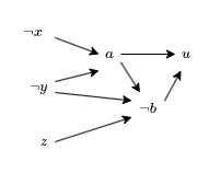
$\neg x$ and $\neg y$ mean $a$ has to be true by unit propagation on the first clause. $a$, $\neg y$ and $z$ mean $\neg b$ has to be true by unit propagation on the second clause. $a$ and $\neg b$ mean $u$ has to be true by unit propagation on the third clause.
A conflict literal $l$ is one for which both $l$ and $\neg l$ appear as nodes in the graph. This is a conflict because $l$ and $\neg l$ cannot be true at the same time. A conflict graph is a subgraph of the implication graph that contains
- exactly one conflict literal $l$
- only nodes that have a path to $l$ or $\neg l$
- incoming edges corresponding to one particular clause only
Consider an edge cut in the conflict graph that has all decision literals on one side of the cut $R$ and the conflict literals on the other side $C$ and all edges across the cut start in $R$ and end in $C$. A conflict clause is the clause obtained by considering all edges $l$ to $l'$ where $l \in R$ and $l' \in C$ and taking the disjunction of all literals $\neg l$. Different learning schemes are used to select which conflict clause to add. Any conflict clause can be inferred by the resolution rule from the existing clauses, so adding conflict clauses does not affect satisfiability.
Conflict-driven clause learning is an algorithm which uses conflicts in implication graphs to decide which clause to add to a formula.
- Select a variable and assign true or false
- Apply unit propagation
- Build the implication graph
- If there is any conflict, derive a corresponding conflict clause and add it to the formula, then non-chronologically backtrack to the decision level where the first assigned variable involved in the conflict was assigned
- Repeat step 1 until all variables are assigned
The solutions considered so far are complete. Monte Carlo methods are incomplete and based on stochastic local search. A simple example is starting with a random truth assignment to the variables. While there are unsatisfied clauses, pick any variable and flop a random literal in it, giving up after some number of trials. For a satisfiable 3-SAT formula with $n$ variables, this algorithm will succeed with probability $\Omega((3/4)^n/n)$ after at most $n$ rounds. If the algorithm is repeated $Kn(4/3)^n$ times for some large enough $K$ then it is almost certain to find a solution. This runs in $O((4/3)^n) \approx O(1.33^n)$ time, which is better than the naive $O(2^n)$ algorithm and the improved $O(1.913^n)$ algorithm but if the formula is not satisfiable, the algorithm will never prove this conclusively.
First-order logic
Every statement in propositional logic is either true or false, it has limited expressive power. First-order logic has the following features
- Propositional connectives and constants
- Quantifiers: $\forall$ and $\exists$
- Variables (not just true or false)
- Relation symbols: $>$, $=$, $p(x)$ where $x$ is prime
- Function symbols: $s(x)$ is the successor of $x$, $x+y$ is the sum of $x$ and $y$
- Constant symbols
For example, "every natural number has a successor" would be denoted $\forall x \exists y(y = s(x))$.
A first order language is determined by specifying
- A finite or countable set $\mathbf{R}$ of relation symbols or predicate symbols, each with some number of arguments
- A finite or countable set $\mathbf{F}$ of function symbols, each with some number of arguments
- A finite or countable set $\mathbf{C}$ of constant symbols
The language determined by $\mathbf{R}$, $\mathbf{F}$ and $\mathbf{C}$ is denoted $L(\mathbf{R}, \mathbf{F}, \mathbf{C})$.
The family of terms of $L(\mathbf{R}, \mathbf{F}, \mathbf{C})$ is the smallest set satisfying the following conditions
- Any variable is a term
- Any constant symbol (member of $\mathbf{C}$) is a term
- If $f$ is a function symbol (member of $\mathbf{F}$) with $n$ arguments and $t_1,...,t_n$ are terms then $f(t_1,...,t_n)$ is a term
An atomic formula of $L(\mathbf{R}, \mathbf{F}, \mathbf{C})$ is any string of the form $R(t_1, ..., t_n)$ where $R$ is a relation symbol (member of $\mathbf{R}$) with $n$ arguments and $t_1, ..., t_n$ are terms. $\top$ and $\bot$ are also taken to be atomic formulae.
The family of formulae of $L(\mathbf{R}, \mathbf{F}, \mathbf{C})$ is the smallest set satisfying the following conditions
- Any atomic formula is a formula of $L(\mathbf{R}, \mathbf{F}, \mathbf{C})$
- If $A$ is a formula, so is $\neg A$
- If $A$ and $B$ are formulae and $\circ$ is a binary connective then $(A \circ B)$ is also a formula
- If $A$ is a formula and $x$ is a variable then $\forall x A$ and $\exists xA$ are also formulae
The free-variable occurrences in a formula are defined as follows
- For an atomic formula, they are all the variable occurrences in that formula
- For $\neg A$ they are the free-variable occurrences in $A$
- For $(A \circ B)$, they are the free-variable occurrences in $A$ and $B$
- For $\forall x A$ or $\exists x A$, they are the free-variable occurrences of $A$ except for occurrences of $x$
If a variable occurrence is not free then it is bound. For example, in the formula $Q(x) \rightarrow \forall x R(x)$ the first occurrence of $x$ is free but the second is bound.
A sentence or closed formula of $L(\mathbf{R}, \mathbf{F}, \mathbf{C})$ is a formula with no free-variable occurrences.
First-order logic semantics
A model for the first-order language $L(\mathbf{R}, \mathbf{F}, \mathbf{C})$ is a pair $\mathbf{M} = (\mathbf{D}, \mathbf{I})$ where
- $\mathbf{D}$ is a non-empty set, called the domain of $\mathbf{M}$
- $\mathbf{I}$ is a mapping, called an interpretation, that associates
- to every constant symbol $c \in \mathbf{C}$, some member $c^\mathbf{I} \in \mathbf{D}$
- to every function symbol $f \in \mathbf{F}$ with $n$ arguments, some $n$-ary function $f^\mathbf{I}: \mathbf{D}^n \rightarrow \mathbf{D}$
- to every relation symbol $R \in \mathbf{R}$ with $n$ arguments, some $n$-ary relation $R^\mathbf{I} \subseteq \mathbf{D}^n$
An assignment in a model $\mathbf{M} = (\mathbf{D}, \mathbf{I})$ is a mapping $\mathbf{A}$ from the set of variables to the set $\mathbf{D}$. $x^\mathbf{A}$ denotes the image of $x$ under $\mathbf{A}$.
Let $\mathbf{M} = (\mathbf{D}, \mathbf{I})$ be a model for the language $L(\mathbf{R}, \mathbf{F}, \mathbf{C})$ and let $\mathbf{A}$ be an assignment in this model. Each term $t$ of the language is assigned a value $t^{\mathbf{I}, \mathbf{A}}$ as follows
- For a constant symbol, $c^{\mathbf{I}, \mathbf{A}} = c^\mathbf{I}$
- For a variable, $x^{\mathbf{I}, \mathbf{A}} = x^\mathbf{A}$
- For a function symbol $f$ with $n$ arguments, $(f(t_1,...,t_n))^{\mathbf{I}, \mathbf{A}} = f^\mathbf{I}(t_1^{\mathbf{I}, \mathbf{A}},...,t_n^{\mathbf{I}, \mathbf{A}})$
For example, consider the language $L(\emptyset, \{s, +\}, \{0\})$ and terms $t_1 = s(s(0) + s(x))$ and $t_2 = s(x+s(x+s(0)))$.
One model of this language is $\mathbf{D} = \mathbb{N}$, $0^\mathbf{I} = 0$, $s^\mathbf{I}$ is the successor function and $+^\mathbf{I}$ is the addition operation. If $\mathbf{A}$ is an assignment such that $x^\mathbf{A} = 3$ then $t_1^{\mathbf{I}, \mathbf{A}} = 6$ and $t_2^{\mathbf{I}, \mathbf{A}} = 9$.
Another model could be $\mathbf{D}$ is the set of all words over the alphabet $\{a,b\}$, $0^\mathbf{I} = a$, $s^\mathbf{I}$ appends $a$ to the end of a word and $+^\mathbf{I}$ is concatenation. If $A$ is an assignment such that $x^\mathbf{A} = aba$ then $t_1^{\mathbf{I}, \mathbf{A}} = aaabaaa$ and $t_2^{\mathbf{I}, \mathbf{A}} = abaabaaaaa$. This shows how the same language can have different semantics under different models and assignments.
Let $\mathbf{M} = (\mathbf{D}, \mathbf{I})$ be a model for the language $L(\mathbf{R}, \mathbf{F}, \mathbf{C})$ and let $\mathbf{A}$ be an assignment in this model. Each formula $\phi$ of $L(\mathbf{R}, \mathbf{F}, \mathbf{C})$ has a truth value $\phi^{\mathbf{I}, \mathbf{A}}$ as follows
- $R(t_1, ..., t_n)^{\mathbf{I}, \mathbf{A}} = \text{true}$ if and only if $(t_1^{\mathbf{I}, \mathbf{A}},...,t_n^{\mathbf{I}, \mathbf{A}}) \in R^\mathbf{I}$
- $\top^{\mathbf{I}, \mathbf{A}} = \text{true}$
- $\bot^{\mathbf{I}, \mathbf{A}} = \text{false}$
- $(\neg X)^{\mathbf{I}, \mathbf{A}} = \neg(X^{\mathbf{I}, \mathbf{A}})$
- $(X \circ Y)^{\mathbf{I}, \mathbf{A}} = X^{\mathbf{I}, \mathbf{A}} \circ Y^{\mathbf{I}, \mathbf{A}}$
- $(\forall x \phi)^{\mathbf{I}, \mathbf{A}} = \text{true}$ if and only if $\phi^{\mathbf{I}, \mathbf{A'}} = \text{true}$ for every assignment $\mathbf{A'}$ that differs from $\mathbf{A}$ by the value assigned to $x$
- $(\exists x \phi)^{\mathbf{I}, \mathbf{A}} = \text{true}$ if and only if $\phi^{\mathbf{I}, \mathbf{A'}} = \text{true}$ for some assignment $\mathbf{A'}$ that differs from $\mathbf{A}$ by the value assigned to $x$
A formula $\phi$ of $L(\mathbf{R}, \mathbf{F}, \mathbf{C})$ is true in the model $\mathbf{M} = (\mathbf{D}, \mathbf{I})$ if $\phi^{\mathbf{I}, \mathbf{A}}$ is true for all assignments $\mathbf{A}$.
A formula is valid if it is true in all models for the language.
A set of formulae $S$ is satisfiable in $\mathbf{M} = (\mathbf{D}, \mathbf{I})$ if there is an assignment $\mathbf{A}$ such that $\phi^{\mathbf{I}, \mathbf{A}}$ is true for all $\phi \in S$.
Formal theorem proving is usually concerned with establishing that a formula is valid. Arbitrary formulae can be turned into sentences by universally quantifying free variables. A sentence $X$ is a logical consequence of a set $S$ of sentences, denoted $S \vDash X$ if $X$ is true in every model in which all the members of $S$ are true.
First-order proof systems
The propositional proof procedures can be extended to prove first-order logic. As well as $\alpha$ and $\beta$ formulae, first-order proof systems use $\gamma$ and $\delta$ formulae as well. $\gamma$ formulae are universally quantified and $\delta$ are existentially quantified.
Universal
| $\gamma$ | $\gamma(t)$ |
|---|---|
| $\forall x \phi$ | $\phi\{x/t\}$ |
| $\neg\exists x \phi$ | $\neg\phi\{x/t\}$ |
Existential
| $\delta$ | $\delta(t)$ |
|---|---|
| $\exists x \phi$ | $\phi\{x/t\}$ |
| $\neg\forall x \phi$ | $\neg\phi\{x/t\}$ |
where $\phi\{x/t\}$ denotes the formula obtained from $\phi$ by replacing the free variable occurrences of the variable $x$ with the term $t$.
Given $L(\mathbf{R}, \mathbf{F}, \mathbf{C})$, let $\mathbf{par}$ be a countable set of constant symbols that are disjoint from $\mathbf{C}$. The elements of $\mathbf{par}$ are called parameters and $L^\mathbf{par}$ is a shorthand for $L(\mathbf{R}, \mathbf{F}, \mathbf{C} \cup \mathbf{par})$.
First-order tableau
For tableau proof, $\gamma$-formulae add new node with $\gamma(t)$ where $t$ is any closed (no variables) term of $L^\mathbf{par}$ and $\delta$-formulae add a new node with $\delta(p)$ where $p$ is a new parameter that has not yet been used in the proof tree. Proofs will be of sentences of $L$, but they use sentences of $L^\mathbf{par}$.
An example tableau proof for $\forall x(P(x) \vee Q(x)) \rightarrow (\exists x P(x) \vee \forall x Q(x))$:
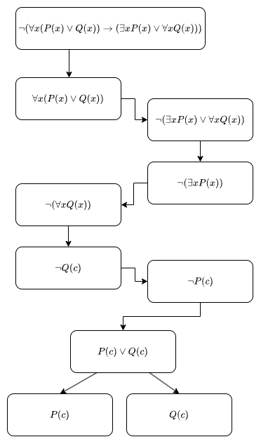
The first four children are derived from alpha expansion. The $\delta$ rule is applied to $\neg(\forall x Q(x))$ with parameter $c$ (this does not have special meaning, it is just a new parameter, it could be called $d$ instead) to give $\neg Q(c)$. The $\gamma$ rule is applied to $\neg(\exists x P(x))$ to give $\neg P(c)$, where $c$ is used as the replacement term. A different term could be substituted but this would not lead to a contradiction. Finally, $\forall x(P(x) \vee Q(x))$ becomes $P(c) \vee Q(c)$ by the $\gamma$ rule. This is then beta-expanded to give a contradiction on both branches. This is a closed tableau, so the original formula is valid.
As before, tableau rules are non-deterministic, but it is usually advantageous to do delta rules before gamma rules as the gamma rules can use the new parameters, making a contradiction easier. It is not possible to strictly apply the $\gamma$ rule, so heuristics are needed instead.
First-order resolution
Resolution works similarly to tableau. $\gamma$ formula are replaced with $\gamma(t)$ and $\delta$ with $\delta(p)$.
The resolution proof for $\forall x(P(x) \vee Q(x)) \rightarrow (\exists x P(x) \vee \forall x Q(x))$ (same as the tableau example) is as follows:
- Take negation: $\left[\neg(\forall x(P(x) \vee Q(x)) \rightarrow (\exists x P(x) \vee \forall x Q(x)))\right]$
- $\alpha$-expansion on 1: $\left[\forall x(P(x) \vee Q(x))\right]$ and $\left[\neg(\exists x P(x) \vee \forall x Q(x))\right]$
- $\alpha$-expansion on 2b: $\left[\neg\exists x P(x)\right]$ and $\left[\neg\forall x Q(x)\right]$
- $\delta$-expansion on 3b: $\left[\neg Q(c)\right]$
- $\gamma$-expansion on 3a: $\left[\neg P(c)\right]$
- $\gamma$-expansion on 2a: $\left[P(c) \vee Q(c)\right]$
- $\beta$-expansion on 6: $\left[P(c), Q(c)\right]$
- Resolution rule on $P(c)$ for 5 and 7: $\left[Q(c)\right]$
- Resolution rule on $Q(c)$ for 4 and 8: $\left[\;\right]$
First-order tableau and resolution are sound and complete. I will not elaborate.
First-order natural deduction
$\gamma$ and $\delta$ formulae can be replaced as with resolution for natural deduction. The natural deduction proof of $\forall x(P(x) \rightarrow Q(x)) \rightarrow (\forall xP(x) \rightarrow \forall x Q(x))$ is as follows
- ┏ $\forall x(P(x) \rightarrow Q(x))$ (assumption)
- ┃┏ $\forall x(P(x)$ (ass.)
- ┃┃┏ $\neg(\forall x Q(x))$ (ass.)
- ┃┃┃ $\neg Q(p)$ ($\delta$-elimination on 3)
- ┃┃┃ $P(p)$ ($\gamma$-elimination on 2)
- ┃┃┃ $P(p) \rightarrow Q(p)$ ($\gamma$-elimination on 1)
- ┃┃┃ $Q(p)$ (modus ponens on 5 and 6)
- ┃┃┗ $\bot$ (negation on 4 and 7)
- ┃┗ $\forall x Q(x)$ (contradiction)
- ┗ $\forall xP(x) \rightarrow \forall x Q(x)$ (impl.)
- $\forall x(P(x) \rightarrow Q(x)) \rightarrow (\forall xP(x) \rightarrow \forall x Q(x))$ (impl.)
First-order natural deduction is sound and complete. Proof is left as an exercise to the reader.
Program verification
Program verification is used to determine if a property holds for a program, denoted $P \vdash \phi$ where $P$ is the program and $\phi$ is the property. An example is x=0; i=1; while(i<=n) { x=x+arr[i]; i=i+1 } $\vdash x = \sum_{i=1}^n \text{arr}[i]$, which verifies that the program finds the sum of the array.
Program verification uses a simple programming language. It consists of three syntactic domains, integer expressions E, boolean expressions B and commands C. The commands include
- assignment,
x = E - composition,
C1; C2 - conditional,
if B then {C1} else {C2} - loops,
while B {C}
The postcondition is the property that must hold when the execution of a program terminates. It is a first-order logic formula referring to program variables which express the conditions formally.
The precondition is the property that program variables must satisfy before the program starts and is also a first-order logic formula. The precondition can also be $\top$, meaning there are no preconditions.
A Hoare triple consists of the precondition, program and postcondition, denoted (|Pre|) Prog (|Post|). This is a logical statement which may be true or false for different values of Pre, Prog and Post.
Examples
- (|$y=1$|) $x = y+1$ (|$x=2$|) is true
- (|$y=1$|) $x = y+1$ (|$x>y$|) is true
- (|$y=1$|) $x = y+1$ (|$x=1$|) is false
- (|$y=1$|) $x = y+1$ (|$z=0$|) is false
From the given precondition we must guarantee that the postcondition is always reached.
Weakest precondition
The weakest precondition (WP) for a program to establish a postcondition is a precondition guaranteeing that the postcondition holds and that it is implied by any other possible precondition, denoted wp(P, Post). It is the minimum requirement for P to successfully reach the postcondition.
Weakest preconditions can be computed formally for each language construct. For assignments, the WP will be the postcondition replaced with the new value. For example, (|?|) x=x+1 (|x>3|) would have WP x+1>3 which is x > 2. Formally, wp(x=E, Post) = Post[x/E] where Post[x/E] is Post with x replaced with E.
Examples
- wp(
x=y,x=6) isx=y[x/y] which isy=6 - wp(
x=1,x>0) isx>0[x/1] which is1 > 0which is $\top$ - wp(
x=0,x>0) isx>0[x/0] which is0 > 0which is $\bot$ - wp(
z=x, $(z \geq x \wedge z \geq y)$) is $(z \geq x \wedge z \geq y)$[z/x] which is $(x \geq x \wedge x \geq y)$ which is $\top \wedge x \geq y$ which is $x \geq y$ - wp(
i=i+1,j=6) isj=6
The WP for composite assignments is wp(P; Q, Post) = wp(P, wp(Q, Post)). For example, wp(x=y+2; y=2*x, x+y>20) is wp(x=y+2, 3*x>20) which is 3*(y+2) > 20 which is 3y > 14.
The WP for conditionals, wp(if B then {C1} else {C2}, Post), is (B $\rightarrow$ wp(C1, Post)) $\wedge$ (¬B $\rightarrow$ wp(C2, Post)) or equivalently (B $\wedge$ wp(C1, Post)) $\vee$ (¬B $\wedge$ wp(C2, Post)).
For example, wp(if x>0 then {y=x} else {y=-x}, $y = \left|x\right|$) gives $(x>0 \rightarrow x = \left|x\right|) \wedge (\neg(x>0) \rightarrow -x = \left|x\right|)$ which is $\top$.
Hoare logic
Any program is a sequence of instructions, Prog = C1; C2; ...; Cn. A proof for Prog shows the preconditions for each command which can then be composed to verify the whole program.
The assignment rule states that (|Post[x/E]|) x = E (|Post|) is a valid Hoare triple and can be introduced wherever an assignment occurs.
The implied rule states that if Pre $\rightarrow$ P then (|P|) Prog (|Post|) can be replaced with (|Pre|) Prog (|Post|). If Q $\rightarrow$ Post then (|Pre|) Prog (|Q|) can be replaced with (|Pre|) Prog (|Post|). This corresponds to strengthening the precondition or weakening the postcondition.
The composition rule states that if (|Pre|) Prog1 (|Mid|) and (|Mid|) Prog2 (|Post|) are valid then (|Pre|) Prog1; Prog2 (|Post|) is valid.
A proof for (|$y = 10$|) x = y-2 (|$x>0$|) would first use the assignment rule to derive (|$y > -2$|) as a precondition which is then used to derive (|$y = 10$|) by the implied rule. Similar to natural deduction proofs, these proofs are built upwards and then read downwards.
The conditional rule states that if (|Pre $\wedge$ B|) C1 (|Post|) and (|Pre $\wedge$ ¬B|) C2 (|Post|) are valid then (|Pre|) if B {C1} else {C2} (|Post|) is valid.
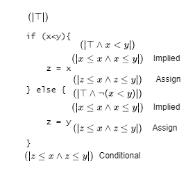
Consider (|$\top$|) if (x<y) then {z=x} else {z=y} (|$z \leq x \wedge z \leq y$|). Applying assignment gives $x \leq x \wedge x \leq y$ for the first branch and $y \leq x \wedge y \leq y$ for the second, which can be simplified to $x \leq y$ and $y \leq x$ respectively. These can be changed to $x < y$ and $\neg(x < y)$ respectively by the implied rule. Given these, the conditional rule can be applied to give $\top$. The proof is shown below.
The loop rule states that if (|B $\wedge$ L|) C (|L|) is valid then (|L|) while B {C} (|¬B $\wedge$ L|) is valid where L is the loop invariant. The loop invariant holds before and after each iteration.