Introduction
Hello! These are my lecture notes for the computer science modules I took while at Warwick.
PLEASE NOTE
I make no guarantee that these notes are correct.
Coverage
This table shows the coverage for each module and how I'd rate the quality.
| Module | Coverage | Quality |
|---|---|---|
| CS118 | IEEE-754, robot maze reference | Ok |
| CS126 | All content, very brief | Ok |
| CS130 | All content, not checked for correctness | Low |
| CS131 | All content, not checked for correctness | Low |
| CS132 | Does not include multithreading and multicore systems, quite brief | Good |
| CS139 | Does not include basics of Python and JS, quite brief | Good |
| CS140 | All content, quite brief | Good |
| CS141 | All content | Good |
| CS241 | All content | Ok |
| CS257 | All content, quite brief | Ok |
| CS258 | All content | Good |
| CS259 | All content | Good |
| CS260 | Does not include P and NP or NP-completeness | Good |
| CS261 | All content, quite brief | Ok |
| CS262 | All content | Good |
| CS263 | All content, very brief | Ok |
| CS313 | All content, quite brief | Good |
| CS325 | Missing quite a lot of Optimisations and Code Generation | Ok |
| CS331 | All content | Good |
| CS349 | Missing everything after type inference and before imperative languages as well as random bits throughout | Ok |
| CS355 | All content | Good |
| CS435 | All content | Good |
CS118 - Programming for Computer Scientists
These notes do not cover basic programming in Java.
IEEE-754
IEEE-754 is the IEEE Standard for Floating-Point Arithmetic.
Floating point numbers can be used to efficiently store very large or very small decimal numbers, similar to standard form/scientific notation but for binary. In Java, these are the float and double types which use 32 and 64 bits respectively.
Floating point numbers consist of a sign bit, exponent and fraction.
- The sign bit is the most significant bit and denotes whether the number is positive (0) or negative (1).
- The exponent describes how much to shift the mantissa. In a 32-bit number it is the most significant 8 bits after the sign bit.
- The mantissa is a binary fraction. The most significant bit represents $2^{-1}$, the second $2^{-2}$ and so on. In a 32-bit number it is the remaining 23 bits.
The value of a floating point number is given by $$ (-1)^{\text{sign bit}} \times 1.(\text{mantissa}) \times 2^{\text{exponent} - \text{bias}} $$ For a 32-bit number the bias is 127, for 64-bit it is 1023.
Floating point to base 10
An example of a 32-bit floating point number is 00111110001000000000000000000000.
The sign bit is 0, the exponent is 01111100 and the mantissa is 01000000000000000000000.
The value of the mantissa is $2^{-2} = 0.25$. The exponent is 124.
The value of the number is therefore given by $(-1)^0 \times 1.25 \times 2^{124-127} = 1 \times 1.25 \times 2^{-3} = 0.15625$
Base 10 to floating point
Consider 38.125.
38.125 is 100110.001 in fixed point binary. Shifting right until the MSB is 1 (normalising) gives 1.00110001. The exponent is 5 as the number has been shifted 5 places to the right. We now have $38.125 = 1.00110001 \times 2^5$, which is of the form $1.(\text{mantissa}) \times 2^{\text{exponent} - \text{bias}}$.
Using 32-bit precision, the exponent is given by 127+5 = 132 = 1000 0100 and the mantissa is 00110001. The sign is 0 so the 32-bit precision floating point representation of 38.125 is 01000010000110001000000000000000.
Special values
These are the special values for a 32-bit precision floating point number.
| Exponent | Mantissa | Value |
|---|---|---|
| 0 | 0 | 0 |
| 255 | 0 | Infinity |
| 0 | not 0 | Denormalised |
| 255 | not 0 | Not a number |
Robot Maze Reference
robot methods
| Name | Arguments | Returns |
|---|---|---|
getRuns | None | int - Number of previous runs the robot has made of the current maze |
look | int - Direction in which to look | int - State of the maze square in the given direction |
face | int - Direction in which to face the robot | void |
setHeading | int - Heading in which to face the robot | void |
getHeading | None | int - Current heading of the robot |
getLocation | None | Point - The x and y coordinates of the robot in the maze |
getTargetLocation | None | Point - The x and y coordinates of the robot's target |
Headings
NORTH, EAST, SOUTH and WEST are referred to as headings.
Headings are used for setHeading and returned by getHeading.
| Name | Value |
|---|---|
NORTH | 1000 |
EAST | 1001 |
SOUTH | 1002 |
WEST | 1003 |
Directions
AHEAD, RIGHT, BEHIND and LEFT are referred to as directions.
Directions are relative to the robot's current heading. Directions are used for
look and face. CENTRE can be used as a null value.
| Name | Value |
|---|---|
AHEAD | 2000 |
RIGHT | 2001 |
BEHIND | 2002 |
LEFT | 2003 |
CENTRE | 2004 |
States
WALL, PASSAGE and BEENBEFORE are referred to as states that a
square in the maze can have. They are returned by look. PASSAGE
means an empty square that has not been visited yet, BEENBEFORE is an
empty square that has been visited.
| Name | Value |
|---|---|
WALL | 3000 |
PASSAGE | 3001 |
BEENBEFORE | 4000 |
Coordinates
Maze coordinates start in the top left corner with $(1,1)$ and finish in
the bottom right corner. The default maze is $15 \times 15$, so the
bottom right corner is $(15,15)$. The coordinates of the robot are given
by getLocation. The coordinates of the target are given by
getTargetLocation. Both of these return a Point object (java.awt.Point), where the x
coordinate is given by p.x and the y by p.y where p is the Point
object.
Important notes
Only headings can be used as the argument for setHeading. Only
directions can be used as the argument for look and face.
IRobot is an interface, robot is an instance of an implementation of
IRobot.
CS126 - Design of Information Structures
These notes are a brief overview of the content for CS126.
Analysis of algorithms
A good algorithm will either be space or time efficient. There are two main ways to test the efficiency of algorithms - experimental and theoretical analysis.
Experimental analysis involves implementing and running an algorithm to determine how much time and space it takes to run. This type of analysis requires the algorithm to be implemented, all types of input to be tested and consistent system performance. In reality, it might not be possible to implement an algorithm, it's almost impossible to consider all types of input and different systems, even those with the same hardware and software, will still not necessarily have consistent run times.
Theoretical analysis uses mathematical methods to determine the asymptotic run time of an algorithm. It uses an abstract description of the algorithm as opposed to a concrete implementation and characterises the time or space complexity as a function of the input size. This allows analysis of an algorithm independent of hardware and software.
Asymptotic analysis
The running time of an algorithm can be split into three cases - best, worst and average. The best case is the minimum time an algorithm takes to run and is not that useful. The worst case is the maximum time an algorithm takes to run for any input. Average case determines how long it typically takes for an algorithm to run, somewhere between best and worst. This can be difficult to determine.
The best, worst and average case can be expressed using asymptotic notation. This ignores constant factors and lower order terms in a function to focus on the main part which affects its rate of growth.
Big-O notation
Big-O notation is used to characterise the worst case complexity of an algorithm. For two functions $f(n)$ and $g(n)$ it can be said that $f(n)$ is $O(g(n))$ if there exists $c>0$ and $N\geq1$ such that $$ f(n) \leq cg(n)\quad\forall n \geq N $$ Big-O notation gives an upper bound on the growth rate of a function as $n$ tends towards infinity. $f(n)$ is $O(g(n))$ means the growth rate of $f(n)$ is no more than that of $g(n)$.
Big-Omega
Big-Omega notation can be used characterise the best case complexity of an algorithm. Formally, $f(n)$ is $\Omega(g(n))$ if there exists $c>0$ and $N\geq 1$ such that $$ f(n) \geq cg(n) \quad \forall n \geq N $$ This is the opposite of big-O and gives the lower bound of the growth rate of $f(n)$.
Big-Theta
Big-Theta notation gives the average case complexity of a function. Formally, $f(n)$ is $\Theta(g(n))$ if there exists $c',c'' > 0$ and $N \geq 1$ such that $$ c'g(n) \leq f(n) \leq c''g(n) \quad \forall n \geq N $$ Big-Theta gives an upper and lower bound on the growth rate of $f(n)$ and is basically a combination of both big-O and big-Omega.
Examples
-
$2n+10$ is $O(n)$ because $$ \begin{aligned} 2n + 10 &\leq cn\\ (c-2)n &\geq 10\\ n &\geq \frac{10}{c-2} \end{aligned} $$ So the constants could be $c=3$ and $N = 10$ or anything else such that the inequality holds.
-
$n^2$ is not $O(n)$ because $$ \begin{aligned} n^2 &\leq cn\\ n &\leq c \end{aligned} $$ and this inequality can't be satisfied because $c$ is a constant.
-
$3n^3 + 20n^2 + 5$ is $O(n^3)$ because $$ \begin{aligned} 3n^3 + 20n^2 + 5 &\leq cn^3\\ 3 + \frac{20}{n} + \frac{5}{n^3} &\leq c \end{aligned} $$ which holds when $c = 4$ and $n \geq 21$ as $$ \frac{20}{n} + \frac{5}{n^3} \leq 1 $$ for all $n \geq 21$.
-
$5n^2$ is $\Omega(n^2)$ because $$ 5n^2 \geq cn^2 $$ for $c = 5$, $n \geq 1$.
-
$5n^2$ is $\Omega(n)$ because $$ 5n^2 \geq cn $$ for $c = 1$ and $n \geq 1$.
-
$5n^2$ is $\Theta(n^2)$ as it is both $O(n^2)$ and $\Omega(n^2)$.
-
$5n^2 + 3n\log n + 2n + 5$ is $O(n^2)$ because $$ 5n^2 + 3n\log n + 2n + 5 \leq (5+3+2+5)n^2 = cn^2 $$ when $c = 15$ and $n \geq 1$.
-
$3\log n + 2$ is $O(\log n)$ because $$ 3\log n + 2 \leq c\log n $$ when $c = 5$ and $n \geq 2$. Note that $n = 1$ will give $\log n = 0$ so $n \geq 2$ is necessary.
-
$2^{n+1}$ is $O(2^n)$ because $$ 2^{n+1} = 2 \cdot 2^n \leq c \cdot 2^n $$ when $c = 2$ and $n \geq 1$.
-
$3n\log n -2n$ is $\Omega(n\log n)$ because $$ 3n \log n - 2n = n\log n +2n(\log n - 1) \geq cn \log n $$ when $c = 1$ and $n \geq 2$.
-
$(n+1)^5$ is $O(n^5)$ because using the binomial expansion $$ (n+1)^5 = \binom{5}{5}n^5 + \binom{5}{4}n^4 + ... + 1 \leq cn^5 $$ when $c = \sum_{n=0}^5 \binom{5}{n}$ and $n \geq 1$.
-
$n$ is $O(n\log n)$ because $$ \begin{aligned} n &\leq cn\log n\\ 1 &\leq c\log n \end{aligned} $$ when $c = 4$ and $n \geq 2$.
-
$n^2$ is $\Omega(n\log n)$ because $$ \begin{aligned} n^2 &\geq cn \log n\\ n &\geq c\log n \end{aligned} $$ when $n \geq 1$ and $c = 1$.
-
$n \log n$ is $\Omega(n)$ because $$ \begin{aligned} n\log n &\geq cn\\ \log n &\geq c \end{aligned} $$ when $c=1$ and $n \geq 10$.
Conclusion
-
$f(n)$ is $O(g(n))$ if $f(n)$ is asymptotically less than or equal to $g(n)$
-
$f(n)$ is $\Omega(g(n))$ if $f(n)$ is asymptotically greater than or equal to $g(n)$
-
$f(n)$ is $\Theta(g(n))$ if $f(n)$ is asymptotically equal to $g(n)$
Recursion
See recursion.
Recursive methods are those that call themselves. A recursive method should have a base case and recursive case. For example, the factorial function has recursive case $f(n) = n \times f(n-1)$ and base case $f(0) = 1$.
Binary search is a recursive divide and conquer search algorithm for sorted data. It chooses a pivot and recursively searches the half of the list based on the difference between the search term and pivot. Binary search has complexity $O(\log n)$. Binary search is an example of linear recursion, where each recursive call makes only one recursive call.
The Fibonacci function, $F(n) = F(n-1) + F(n-2)$ uses binary recursion, as each call makes two recursive calls. A function making more than two recursive calls is said to use multiple recursion.
Data structures
Abstract data types and data structures
- An abstract data type (ADT) is a description of a data structure and its methods, like a Java interface but for a data structure instead of a class.
- A data structure is a concrete implementation of an ADT.
Arrays
Arrays are fixed size, contiguous blocks of allocated memory. Access is $O(1)$ and insertion is $O(n)$.
Linked lists
A linked list consists of nodes which point to the next node and possibly the previous as well.
Singly-linked list
Each node in a singly-linked list has a value and a pointer to the next node and not the previous. There is also a pointer to the head and tail of the list. Access, insertion and deletion are $O(n)$, although insertion and access at the head or tail is $O(1)$. Unlike arrays the linked list is dynamically sized.
Doubly-linked list
Each node points to the next and previous node. The doubly-linked list can be traversed forwards or backwards.
Stacks
A stack is a LIFO data structure. The stack ADT has pop and push methods
to remove the top element and insert an element at the top respectively.
Stacks can be implemented using arrays and each operation is $O(1)$ but
the size is fixed.
Queues
A queue is FIFO data structure. The ADT has enqueue and dequeue methods
for adding to and removing from the queue respectively. The queue can be
implemented with an array. All operations are $O(1)$, but the size is
fixed.
Lists
The list ADT has support for insertion and deletion at arbitrary
positions. It has size, set, get, add and remove methods. An array based
list needs to grow when its backing array gets full. The amortised time
(average time for each operation) of an insertion is better when
doubling the size than increasing the size by a constant factor.
A positional list is a list where the position of an item is relative to the others. This can be implemented with a doubly-linked list.
Maps
Maps are a searchable collection of key-value pairs. Maps support insertion, deletion and searching. Keys must be unique. The key is hashed and divided by the length of the backing structure to give the index of the value.
Hash collisions
Sometimes different keys will map to the same index. This is called a collision and there are two ways to deal with them. The first is separate chaining, where each location is a linked list and if two items have the same index then only the linked list has to be traversed to find it. The other solution is linear probing, where the item is placed in the next vacant adjacent cell. If the hash function does not distribute values well then both methods will become more inefficient. For separate chaining the list will become longer and take longer to traverse, for linear probing more indices will have to be traversed to find a vacant one. The best case for a map is $O(1)$, but with collisions on every element this can be as bad as $O(n)$.
Sets
A set is a collection of distinct, unordered elements. Sets support efficient membership tests and union, intersection and subtraction operations.
Sorting
Generic merge
The generic merge algorithm is used to sort two ordered lists.
public static <E extends Comparable<E>> E[] genericMerge(E[] a, E[] b){
        E[] result = (E[])new Comparable[a.length + b.length];
        int ri = 0, ai = 0, bi = 0;
        // While both lists contain items
        while(!(ai == a.length || bi == b.length)){
            // Compare the current items
            if(a[ai].compareTo(b[bi]) > 0){
                // Add b to the result
                result[ri++] = b[bi++];
            } else{
                // Add a to the result
                result[ri++] = a[ai++];
            }
        }
        // Add the remainder of a
        while(ai < a.length){
            result[ri++] = a[ai++];
        }
        // Add the remainder of b
        while(bi < b.length){
            result[ri++] = b[bi++];
        }
        // Return the result
        return result;
    }
Merge sort
Merge sort is a divide and conquer sorting algorithm. It takes the list, recursively splits it until left with singletons and then uses the generic merge algorithm above to merge the sorted lists.
private static <E> E[] mergeSort(E[] list){
    int size = list.length;
    if(size <= 1){
        // Return singleton or empty list for merging
        return list;
    } else{
        // Find middle index
        int pivot = Math.floorDiv(size, 2);
        // Create lists for two halves
        Object[] left = new Object[pivot];
        Object[] right = new Object[size-pivot];
        // Copy list to halves
        System.arraycopy(list, 0, left, 0, pivot);
        System.arraycopy(list, pivot, right, 0, size-pivot);

        // Recursively merge sort halves
        left = mergeSort((E[])left);
        right = mergeSort((E[])right);
        // Return merged sorted lists
        return genericMerge((E[])left, (E[])right);

    }
}
Merge sort has time complexity $O(n\log n)$.
Quick sort
Quick sort is a randomised divide and conquer sorting algorithm. It chooses a random pivot, then splits the list into items smaller and larger than the pivot, then does the same for each of those lists until every item has been a pivot. The worst case of quick sort occurs when the random pivot is not ideal every time which has complexity $O(n^2)$. The average case is $O(n\log n)$.
Selection sort
Selection sort can be implemented using an unsorted priority queue. It
needs $n$ insertions and $O(n^2)$ removeMin calls, giving an overall run
time of $O(n^2)$.
Insertion sort
Insertion sort uses a sorted priority queue. It still has $O(n^2)$ run time but may perform better than selection sort.
Heaps and priority queues
Priority queue
A priority queue is a queue in which each element is assigned a
priority. The priority queue ADT has insert, removeMin and min methods
for insertion, removing the item with the lowest priority and accessing
the item with the lowest priority respectively. Priority queues can be
used for sorting by inserting elements with priority equal to value and
then removing.
Heap
A heap is a binary tree which stores keys and satisfies the heap-order property. The heap-order property states that every child node is less than or equal to it's parent. The first node in a heap is the root and the last node is the rightmost node of maximum depth. A heap storing $n$ items has height $O(\log n)$.
A priority queue can be implemented using a heap. Each node has the priority as a key where a smaller key means a higher priority and the root node holds the highest priority key.
An item can be inserted into a priority queue heap in the deepest, rightmost part of the heap. The heap order can then be restored using the upheap algorithm. This swaps the new node with its parent until it is smaller than its parent. This runs in $O(\log n)$.
The highest priority item will be the root. When the root is removed, the root is replaced with downheap algorithm. The largest child of a node is swapped with it until it is larger than all of its children.
A heap-based priority sort has run time $O(n \log n)$ because it needs $n$ calls of $O(\log n)$ for each insertion and $n$ calls of removeMin which takes $O(\log n)$ each.
Trees
A graph is a collection of nodes and edges. A tree is a connected, acyclic, undirected graph. This means there is a path between every pair of distinct nodes, there are no cycles and you can go either way along an edge. A binary tree is one in which every node has at most 2 children.
Traversals
Any tree can be traversed in 2 ways - pre-order and post-order. A binary tree can also be traversed in-order.
Pre-order
In a pre-order traversal, the nodes are visited from top to bottom, left to right.
algorithm preOrder(v)
    print(v)
    for each child w of v
        preOrder(w)
Post-order
In a post-order traversal, the nodes are visited from bottom to top, left to right.
algorithm postOrder(v)
    for each child w of v
        postOrder(w)
    print(v)
In-order
In a pre-order traversal, the nodes are visited from top to bottom, left to right.
algorithm inOrder(v)
    if v.left exists
        inOrder(v.left)
    print(v)
    if v.right exists
        inOrder(v.right)
Decision trees
A decision tree is a binary tree in which each internal node is a question and each external node is an outcome. Decision trees can be used to find the lower bound for a sorting algorithm. If each external node in the tree is a possible ordering of the elements there must be $n!$ (from the definition of permutations) of them, giving a tree with height $\log(n!)$. This means any comparison based sorting algorithm takes at least $\log(n!)$ time. It can be shown that this means any comparison-based sorting algorithm must run in time $\Omega(n\log n)$, so $O(n \log n)$ is the most efficient comparison-based sorting algorithm time complexity.
Binary search tree
A binary search tree (BST) is a binary tree containing keys on the internal nodes and nothing on external nodes. For each internal node, the keys in the left subtree are less than its key and the keys in the right are greater than. An in-order traversal of the tree gives the keys in increasing order.
Search
To find a key in a BST, start at the root. If the key is equal to the root key, the item is found, if it is less than recursively search the left subtree, if it is greater than recursively search the right subtree. If an external node is reached the key is not found.
Insertion
Search the tree for the new key, then replace the external node with a new node containing the new key and give it two empty children.
Deletion
Search for the key to remove. If it has no internal children just replace it with an empty node. If it has one internal child, replace it with that child. If the node has two internal children, find the next node using an in-order traversal, then replace the removed node with it.
Performance
Space $O(n)$, height is best case $O(\log n)$ worst case $O(n)$, and search, insertion and deletion are $O(h)$ where $h$ is the height.
AVL trees
AVL trees are balanced binary trees. They are balanced regardless of insertion order. It achieves this using the height balance property, which states the difference in height between internal nodes and their internal children is at most 1. The height of an AVL tree storing $n$ keys is $O(\log n)$.
Rotations
Inserting into an AVL tree works the same as a binary tree, but if the insertion makes the tree unbalanced it needs to be rotated to balance it again. Rotations allow re-balancing the tree without violating the BST property.
Performance
AVL trees take $O(n)$ space and searching, insertion and removal take $O(\log n)$ time. A single restructuring takes $O(1)$ time with a linked-structure binary tree.
Graphs
-
A graph is a collection of nodes/vertices and edges.
-
Edges on a graph can be directed or undirected.
-
Vertices are adjacent if they are connected by an edge.
-
Edges are incident to a vertex if they are connected to it.
-
The degree of a vertex is the number of edges connected to it.
-
A path is a sequence of connected vertices and edges in a graph.
-
A cycle is a path where the start and end vertices are the same.
-
An connected, undirected, acyclic graph is a tree.
-
The sum of the degrees is twice the number of edges.
-
A subgraph is a graph which contains a subset of the edges and vertices in a graph.
-
A spanning subgraph is a subgraph which contains all vertices in the original graph.
-
A forest is a collection of trees.
-
A spanning tree of a connected graph is a spanning subgraph which is also a tree.
Graph traversals
Depth first search
Depth first search (DFS) is a graph traversal where the graph is traversed as deeply as possible, then across.
Breadth first search
Breadth first search (BFS) traverses across a graph, then down.
CS130 - Mathematics for Computer Scientists I
These are just my unedited lecture notes. I wasn't particularly good at CS130 so some of it is probably wrong.
Sets, sequences and functions
Introduction to sets
A set is a collection of objects. Sets are written in curly brackets. For example, the set of integers:
$$ \mathbb{Z} = \{0,1,-1, 2, -2, ...\} $$ To say an item belongs to a set you use $\in$, which means "belongs to" or "is a member of". For example, $12\in\mathbb{Z}$ because 12 is an integer.
The ordering of sets is not important. $\{1,0\}$ is the same as
$\{0,1\}$.
Sets with different numbers of the same item are the same. $\{1,1,1,2\}$
is the same as $\{1,2,2\}$ is the same as $\{1,2\}$.
To show one set is a subset of another, you can use $\subseteq$. For
example, $\{1,2,3,4\}\subseteq\mathbb{Z}$ as every item in $\{1,2,3,4\}$
is also in $\mathbb{Z}$.
Note that
$\mathbb{N}\subseteq\mathbb{Z}\subseteq\mathbb{Q}\subseteq\mathbb{R}$.
Also note that $\mathbb{Z}$ includes 0.
The number of items in a set (it's cardinality) $A$ is expressed as $|A|$. For example, $|\{1,2,3,4,5\}|=5$.
Specifying sets
You can specify a set using set builder notation. For example, the set of integers greater than 7 can be expressed
as $\{n\in\mathbb{Z}:n>7\}$, or the set of integers such that
$n > 7$.
The set of square integers can be expressed as $\{n^2:n\in\mathbb{Z}\}$.
This means the set of $n^2$ such that $n$ is an integer.
The set $\{(-1)^k:k\in\mathbb{Z}\}$ is the set of $(-1)^k$, such that
$k$ is an integer. For $k = 0$, $(-1)^0 = 1$, for $k = 1$,
$(-1)^1 = -1$, for $k = 2$, $(-1)^2 = 1$.
This pattern will repeat, so $\{(-1)^k:k\in\mathbb{Z}\}=\{1,-1\}$.
An empty set can be shown using $\emptyset$ or $\{\:\}$.
Sets with only one element ($|$set$| = 1$) are called singletons.
Finite sequences
Let $A = \{a, b, c\}$. $A^2 = \{(a,a),(a,b),(a,c),...,(c,c)\}$.
($(a,a)$ is a tuple that represents a sequence)
This can be generalised to $A^n =$ the set of all sequences of length
$n$ of elements of $A$.
If $A$ is finite, $|A^n| = |A|^n$.
The general form of $A^n$ is
$$ A^n = \{(a_1,...,a_n):a_1\in A, a_2\in A, ..., a_n\in A\} $$ This means the set of sequences from $a_1$ to $a_n$ such that $a_1$ to $a_n$ belong to $A$. For example, the set $\mathbb{Z}^2$ can be expressed as
$$ \mathbb{Z}^2 = \{(x,y):x\in \mathbb{Z}, y \in \mathbb{Z}\} $$
Introduction to functions
If there is a rule that assigns to each element $x\in X$ an
unambiguously determined element of the set Y, then it is a function
from X to Y.
This can be denoted as $f: X \to Y$.
$X$ is called the domain and $Y$ is called the co-domain.
Take $f(x) = x^2 - 3$ for example. For each value of $x$,
$x\mapsto x^2-3$. ($\mapsto$ means maps to).
This can then be expressed as $f:\mathbb{R}\to \mathbb{R}$, as each real
number is mapped to another real number.
Another example is $f(x) = \sqrt{x}$. This will map any positive real number to a positive real number, so $f:\mathbb{R}\geq 0 \to \mathbb{R} \geq 0$.
The left set, $X$, is the domain, and each item in the set ($x\in X$) is
shown to map to a value in the right set, $Y$, which is the co-domain.
It is possible for two items from $X$ to map to one item in $Y$.
This shows clearly how the function maps every item in set $X$ to set
$Y$.
It can be said that $f(x)$ is the image of $x$ under $f$ and that $f$
maps $X$ to $Y$.
More examples of functions
Consider the following functions
-
$f_1(x)=\frac{1}{x}$
-
$f_2(x)=\sqrt{x}$
-
$f_3(x) = \pm \sqrt{x^2+1}$
Which of these are functions from $\mathbb{R}$ to $\mathbb{R}$?
-
This is not a function from $\mathbb{R}$ to $\mathbb{R}$ as $f(0)$ is undefined, so there is not a mapping of every $x$ to some $f(x)$.
-
This is not a function from $\mathbb{R}$ to $\mathbb{R}$ as negative numbers map to complex numbers, which are not in the set $\mathbb{R}$.
-
This is not a function from $\mathbb{R}$ to $\mathbb{R}$, as it maps to two values, not one.
Logic
Introduction to propositional logic
A proposition is a statement that asserts something. Propositional logic abstracts propositions with propositional variables or atomic propositions. $p$ or $q$ are common variables for atomic propositions.
Compound propositions are made up of atomic propositions or other
compound propositions.
Some examples:
| Compound proposition | Name |
|---|---|
| $\neg p$ | negation (logical not) |
| $p \wedge q$ | conjunction (logical and) |
| $p \vee q$ | disjunction (logical or) |
Boolean functions and truth tables
Boolean functions are of the form $B^n \to B$, where
$B = \{True, False\}$.
Example:
$$
\begin{aligned}
& B^2 = \{FF,FT,TF,TT\}\\
& \text{A function that could map } B^2 \text{ to } B \text{ is } h(x,y) = x \vee y \text{ where } x,y \in B.
\end{aligned}
$$
You can draw a truth table to show the possible outputs
of a boolean function.
Here is the truth table for $x \vee y$:
| $x$ | $y$ | $f(x,y)$ |
|---|---|---|
| $F$ | $F$ | $F$ |
| $F$ | $T$ | $T$ |
| $T$ | $F$ | $T$ |
| $T$ | $T$ | $T$ |
$x \to y$ shows material implication. This means $x$ implies $y$. It is equivalent to $(\neg x) \vee y$.
| $x$ | $y$ | $x \to y$ |
|---|---|---|
| $F$ | $F$ | $T$ |
| $F$ | $T$ | $F$ |
| $T$ | $F$ | $T$ |
| $T$ | $T$ | $T$ |
Logical equivalence and laws of propositional logic
Boolean functions and logical equivalence
Propositions $P$ and $Q$ are logically equivalent if the proposition
$P \Leftrightarrow Q$ is a tautology.
The truth table for $x \Leftrightarrow y$:
| $x$ | $y$ | $x \Leftrightarrow y$ |
|---|---|---|
| $F$ | $F$ | $T$ |
| $F$ | $T$ | $F$ |
| $T$ | $F$ | $F$ |
| $T$ | $T$ | $T$ |
Both values have to be the same for $x \Leftrightarrow y$ to be true. $\Leftrightarrow$ shows equivalence.
A proposition is a tautology if it is true regardless of the values of
atomic propositions. A tautology is a proposition which is always true.
$P \equiv Q$ shows two propositions, $P$ and $Q$, are equivalent.
Laws of propositional logic
| Rule | Name |
|---|---|
| $(x\vee y)\vee z \equiv x \vee y\vee z)$ | associativity |
| $(x\wedge y)\wedge z \equiv x\wedge (y\wedge z)$ | associativity |
| $x \vee y \equiv y \vee x$ | commutativity |
| $x \wedge y \equiv y \wedge x$ | commutativity |
| $x \vee \text{False} \equiv x$ | identity |
| $x \wedge \text{True} \equiv x$ | identity |
| $x \vee x \equiv x$ | idempotence |
| $x \wedge x \equiv x$ | idempotence |
| $\neg (x \vee y) \equiv \neg x \wedge \neg y$ | De Morgan's law |
| $\neg(x \wedge y) \equiv \neg x \vee \neg y$ | De Morgan's law |
| $\neg (\neg x) \equiv x$ | double negation |
| $x \vee \neg x \equiv \text{True}$ | excluded middle |
| $x \wedge \neg x \equiv \text{False}$ | excluded middle |
| $x \vee (x \wedge y) \equiv x$ | absorption |
| $x \wedge (x \vee y) \equiv x$ | absorption |
| $x \wedge (y \vee z) \equiv (x \wedge y) \vee (x \wedge z)$ | distributivity |
| $x \vee (y \wedge z) \equiv (x \vee y) \wedge (x \vee z)$ | distributivity |
| $x \vee \text{True} = \text{True}$ | annihilation |
| $x \wedge \text{False} \equiv \text{False}$ | annihilation |
Alternative notation
Logical AND: $x \wedge y$, $x \& y$, $x \cdot y$, $xy$.
Logical NOT: $\neg x$, $\bar{x}$.
Predicates and quantifiers
Introduction to predicates and quantifiers
A predicate is a statement about a variable which can be true or false but not both. For example $p(u)$ is a predicate and $u$ is a variable.
Variables can be bound by quantifiers.
| Quantifier | Meaning |
|---|---|
| $\forall$ | "For all" |
| $\exists$ | "There exists" |
For example, $p(u): u > 2$ and $u<17$ is a predicate. For
$u \in \mathbb{Z}$, $p(0)$ is false and $p(15)$ is true.
$\exists u \;p(u)$ is true, as there exists an integer between 2 and 17,
whereas $\forall u \:p(u)$ is false as it is not true for all integers.
When a quantifier applies to a variable, the variable is said to be bound. For example, $p(x): x^2 = 2$ is a predicate and the variable $x$ is not bound, so it is free. If it is said that $\exists x \in \mathbb{Z} \; p(x)$ then the variable is now bound to a quantifier and is no longer free.
It is possible for predicates to have multiple variables. $p(x,y): x^2 - y^2 = (x-y)(x+y)$, for example, has 2 variables. Given that $x,y \in \mathbb{Z}$, It can be said that $\exists x \exists y \; p(x,y)$ and also $\forall x \forall y \; p(x,y)$ as the statement holds true for all integers $x$ and $y$.
Alternation of quantifiers
$q(u,v):|u-v|=1$, $u,v \in \mathbb{Z}$.
$\forall u \; \exists v \; q(u,v)$ is true, as for every integer $u$
there exists another integer $v$ with a difference of 1.
$\exists v \; \forall u \; q(u,v)$ is false, as there does not exist a
single integer $v$ which has a difference of 1 with every number $u$.
Despite having the same quantifiers, the order is important.
Laws of predicate logic
Quantification over finite sets
Consider a finite set of integers $A = \{1,2,3,4,5,...,n\}$.
$\forall x \in A\; P(x) \equiv P(1) \wedge P(2) \wedge ... \wedge P(n)$
and
$\exists x \in A \; P(x) \equiv P(1) \vee P(2) \vee ... \vee P(n)$ where
$P(x)$ is a predicate.
Another example:
$S = \{a,b,c\}$
$\forall x \; \exists y \; f(x,y)$
You can expand this out using the methods above:
$(\exists y \; f(a,y))\wedge(\exists y \; f(b,y))\wedge(\exists y \; f(c,y))$
Then applying the method again:
$(f(a,a) \vee f(a,b) \vee f(a,c)) \wedge$
$(f(b,a) \vee f(b,b) \vee f(b,c)) \wedge$
$(f(c,a) \vee f(c,b) \vee f(c,c))$
Working with quantifiers
$\forall x \; \text{True} \equiv \text{True}$
$\exists x \; \text{True} \equiv \text{True}$
$\forall x \; \text{False} \equiv \text{False}$
$\exists x \; \text{False} \equiv \text{False}$
$\forall x \; (P(x) \wedge Q) \equiv (\forall x \; P(x)) \wedge Q$
$\exists x \; (P(x) \wedge Q) \equiv (\exists x \; P(x)) \wedge Q$
These are interchangeable with $\vee$.
De Morgan's laws for quantifiers:
$\neg(\forall x \; P(x)) \equiv \exists x \; \neg P(x)$
$\neg(\exists x \; P(x)) \equiv \forall x \; \neg P(x)$
$\forall x \; (P(x) \wedge Q(x)) \equiv (\forall x\; P(x))\wedge (\forall x \; Q(x))$
This will not work for $\exists$, as $\exists x \; (P(x) \wedge Q(x))$
means there exists an $x$ such that both $P(x)$ and $Q(x)$ are true, but
if you try to split it like before you get
$(\forall x\; P(x))\wedge (\forall x \; Q(x))$ and there is a
possibility the values for $x$ will be different but still true for both
predicates.
There is a similar rule for disjunction ($\vee$). This only works with $\exists$ in both directions. $\exists x\; (P(x) \vee q(x)) \equiv (\exists x \; P(x)) \vee (\exists x \; Q(x))$. This will work with $\forall$ in the backward direction for the same reason as the last one.
Uniqueness
Suppose you want to find if only one item in a set satisfies a predicate. To express "at least one item satisfies the predicate" you can use $\exists x \in S\; P(x)$ - there exists an $x$ such that $P(x)$. This checks there is an item that satisfies the predicate, but not that it is the only one - there could be multiple.
To check it is unique, you can use $\forall y \in S \; \forall z \in S \; [(P(y)\wedge P(z))\to y = z]$. This says for all $y$ and $z$ which belong to $S$, if both satisfy the predicate it is implied that they are equal. Combining the checks for an item which satisfies $P(x)$ and is unique, you get $(\exists x \in S\; P(x)) \wedge (\forall y \in S \; \forall z \in S \; [(P(y)\wedge P(z))\to y = z])$.
The second part can be simplified using the previously mentioned rules. $(P(y)\wedge P(z)) \to y=z$ can be changed into $\neg P(y) \vee \neg P(z) \vee y=z$ because implication is logically equivalent to $\neg x \vee y$. Now we have $(\exists x \in S\; P(x)) \wedge (\forall y \in S \; \forall z \in S \; [\neg P(y) \vee \neg P(z) \vee y=z])$.
Algebra of sets
Set-theoretic operations
- $A \cup B$ is the union of $A$ and $B$.
- $A \cup B = \{x:x \in A \vee x \in B\}$.
- $A \cap B$ is the intersection of $A$ and $B$.
- $A \cap B = \{x:x \in A \wedge x \in B \}$.
- $A \setminus B$ is the set difference.
- $A \setminus B = \{x:x\in A \wedge x \notin B\}$.
- $A \bigtriangleup B$ is the symmetric difference.
- $A \bigtriangleup B = (A \setminus B) \cup (B \setminus A)$.
The laws of Boolean logic (associativity, distributivity, idempotence, commutativity, De Morgan's, etc.) also apply to sets, where $\cup$ is equivalent to $\vee$, $\cap$ is equivalent to $\wedge$ and an overline is used to show negation ($\overline{A}$).
Set difference proof
Prove $A \bigtriangleup B = (A\setminus B) \cup (B \setminus A) = (A \cup B) \setminus (A \cap B)$:
-
Let $x \in (A \setminus B) \cup (B \setminus A)$.
-
Consider the case $x \in A \setminus B$: $x \in A$ and $x \notin B$.
If $x\in A$ then $x \in A \cup B$. If $x \notin B$ then $x \notin A \cap B$. Combining the two expressions using the definition of $A \setminus B$ gives $x \in (A \cup B) \setminus (A \cap B)$. -
The same can be said when $x \in B \setminus A$:
$x \in B$, $x \notin A$, $x \in A \cup B$, $x \notin A \cap B$, $x \in (A \cup B) \setminus (A \cap B)$.
This has shown that $(A\setminus B) \cup (B \setminus A) \in (A \cup B) \setminus (A \cap B)$, but not the other way round.
-
-
Let $x \in (A \cup B) \setminus (A \cap B)$.
Using the set difference, $x \in (A \cup B)$ and $x \notin (A \cap B)$.
If $x \in (A \cup B)$, $x \in A$ or $x \in B$. Both can not be true or $A \cap B$ would be true, but $x \notin A \cap B$.
This means either $x \in A \wedge x \notin B$ or $x \in B \wedge x \notin A$.
Therefore, $x \in A \setminus B$ or $x \in B \setminus A$ by definition of set difference.
This has shown that $(A\cup B)\setminus (A \cap B) \in (A \setminus B) \cup (B \setminus A)$.
It has now been shown that both $(A\setminus B) \cup (B \setminus A) \in (A \cup B) \setminus (A \cap B)$ and $(A\cup B)\setminus (A \cap B) \in (A \setminus B) \cup (B \setminus A)$. Therefore the sets are equal.
Expressions with indices
To define multiple sets, where each is the set of integers from $i$, you can use $A_i = \{x \in \mathbb{Z} : x \geq i\}$. To express the union of all of those sets ($A_1 \cup A_2 \cup A_n$), you can use a big $\cup$, similar to series notation: $\displaystyle\bigcup_{i=1}^{n}{A_i}$ and similarly $\displaystyle\bigcap_{i=1}^{n}{A_i}$ for intersection. Similarly to how the sum of natural numbers can be expressed in terms of $n$, the same can be done for sets. Using $A_i = \{x \in \mathbb{Z} : x \geq i\}$ as an example:
| Notation | Value | Reason |
|---|---|---|
| $\displaystyle\bigcup_{i=1}^{n}{A_i}$ | $A_1$ | The intersection of all sets will be $A_1$ because it is the largest set. |
| $\displaystyle\bigcap_{i=1}^{n}{A_i}$ | $A_n$ | $A_n$ is the only set which is a subset of the sets before it, so is the value of the intersection. |
The values will change dependent on the definition of $A_i$.
It is also possible to make a general form for infinity:
$$ \begin{aligned} & \bigcup_{i=1}^{\infty} A_i = \{x:x \in A_i \text{ for some } i \in \mathbb{N} \}\\ & \bigcap_{i=1}^{\infty} A_i = \{x:x \in A_i \text{ for all } i \in \mathbb{N} \} \end{aligned} $$
Using $A_i = \{x \in \mathbb{Z} : x \geq i\}$ as an example again:
$$ \begin{aligned} & \bigcup_{i=1}^{\infty} A_i = A_1\\ & \bigcap_{i=1}^{\infty} A_i = \emptyset \end{aligned} $$ The union to infinity is the same as the the union to $n$. The intersection is different, as the set of integers not contained in the set of integers is the empty set.
Power sets and Cartesian products
Power set
The power set is the set of all subsets of a set.
| Set | Power set |
|---|---|
| $S_1 = \emptyset$ | $2^{S_1} = \{\emptyset\}$ |
| $S_2 = \{a, b\}$ | $2^{S_2} = \{\emptyset, \{a\}, \{b\}, \{a,b\}\}$ |
| $S_3 = \{1\}$ | $2^{S_3} = \{\emptyset, \{1\}\}$ |
In general, the power set of a set $S$ is denoted $2^S$ and is the set of all subsets of $S$. A power set of a finite set $S$ contains $2^{|S|}$ items.
Cartesian product and ordered pairs
The Cartesian product of two sets, $A \times B$, is the set of all ordered pairs $(a,b)$ where $a \in A$ and $b \in B$: $A \times B = \{(a, b) : a \in A, b \in B\}$.
Take two sets, $A = \{k,l,m\}$ and $B = \{q,r\}$. The Cartesian product of these sets would be $\{(k, q), (k, r), (l, q), (l, r), (m, q), (m, r)\}$ . Note that the first item in the sequences is from $A$ and the second is from $B$. For $B \times A$, the pairs will be swapped.
Proof
Direct proof
Direct proofs use assumptions to show something is true. Consider the statement "If $2^A \subseteq 2^B$ then $A \subseteq B$.". To prove this, we can take an arbitrary $x \in A$. It can then be said that $\{x\} \in 2^A$, as $\{x\}$ must be part of the power set of $A$. Since $2^A \subseteq 2^B$, $\{x\} \in B$, so $x \in B$. This shows that $A \subseteq B$ as $x$ is in both. This proof made use of assumption $2^A \subseteq 2^B$ to show $A \subseteq B$.
Using cases
Another way to prove something is by considering all the cases. Take the statement "$1+((-1)^n)(2n-1)$ is a multiple of 4 $\forall n \in \mathbb{Z}$". The value of $(-1)^n$ depends on whether the number is even or odd.
-
In the case the number is even, $(1+1(2n-1) = 2n$. As $n$ is even, we can substitute $n = 2k, k\in \mathbb{Z}$. This gives $4k$, which is divisible by 4.
-
In the case the number is odd, $(1-1(2n-1) = 1-2n+1 = 2-2n$. As $n$ is odd, $n = 2k-1$. This gives $2-2(2k-1) = 2-4k+2 = 4-4k = 4(1-k)$, so it's divisible by 4 when $n$ is odd.
As all $n\in \mathbb{Z}$ must be either odd or even, it has been shown that $1+((-1)^n)(2n-1)$ is a multiple of 4 $\forall n \in \mathbb{Z}$.
Proof by contrapositive
Proof by contrapositive uses the opposite of the statement to show that it isn't true, therefore the original statement was true. Consider "If $7x+9$ is even, then $x$ is odd." Assuming $x$ is even (opposite of the original statement), $x = 2m$. This gives $7(2m)+9 = 14m + 9 = 2(7m+4)+1$ which is always odd, so $7x+9$ is not even when $x$ is even. Therefore $x$ must be odd. Note this could also be proven by direct proof.
Proof by contradiction
Proof by contradiction assumes the opposite of something. Take the statement $\sqrt{2} \notin \mathbb{Q}$. Assuming $\sqrt{2} \in \mathbb{Q}$ (the opposite), it can be defined as a fraction of two integers in it's simplest form. $\sqrt{2} = \frac{m}{n}, m,n \in \mathbb{N} \setminus \{0\}$. Squaring both sides gives $2 = \frac{m^2}{n^2}$, so $2n^2 = m^2$. This means $m$ must be even, so let $m=2k$. $2n^2 = (2k)^2, 2n^2 = 4k^2, n^2 = 2k^2$. This means $n^2$ must be even, therefore $n$ must be even. If both $n$ and $m$ are even, then the fraction is not in it's simplest form. This contradicts $\sqrt{2} \in \mathbb{Q}$, so $\sqrt{2} \notin \mathbb{Q}$.
Whereas proof by contrapositive only takes the opposite of the last part of the statement, proof by contradiction takes the opposite of the whole statement.
Non-constructive proof
Theorem:
"$\exists \: x,y \in \mathbb{R} \setminus \mathbb{Q}:x^y \in \mathbb{Q}$"
(There exists an $x$ and $y$ which belong to the set of irrational
numbers such that $x^y$ is rational.)
Consider $a = \sqrt{2}^{\sqrt{2}}$ and $b = \sqrt{2}$. Therefore
$a^b = (\sqrt{2}^{\sqrt{2}})^{\sqrt{2}}=\sqrt{2}^{\sqrt{2}\times \sqrt{2}} = \sqrt{2}^2 = 2$.
This presents two cases:
-
If $a,b \in \mathbb{R} \setminus \mathbb{Q}$, then $x=a, y=b$. (If $a$ and $b$ are irrational, then it has been shown that $a^b$ is rational)
-
If $a \in \mathbb{Q}$ then $x=\sqrt{2}, y=\sqrt{2}$. (If $a$ turns out to be rational, then it is equal to $\sqrt{2}^{\sqrt{2}}$, where both are irrational)
Only one of the two cases can be true, 1 fails if 2 is true and vice versa, but both show that $x^y$ is rational when $x$ and $y$ are irrational, so the theorem is still proven regardless of which is true.
Logic in proof
Example 1
$$ \begin{aligned} x \wedge (\neg x \vee y) &\equiv x \wedge y \\ x \vee (\neg x \wedge y) &\equiv x \vee y \end{aligned} $$
Proof:
$$ \begin{aligned} \text{1. For all } x, y \in \{T, F\}^2, x \wedge (\neg x \vee y) &= (x \wedge \neg x) \vee (x \wedge y) & \text{(Distributivity)}\\ &= F \vee (x \wedge y) & \text{(Excluded middle)}\\ &= (x \wedge y) \blacksquare & \text{(Identity)}\\ \text{2. For all } x, y \in \{T, F\}^2, x \vee (\neg x \wedge y) &= (x \vee \neg x) \wedge (x \vee y) & \text{(Distributivity)}\\ &= T \wedge (x \vee y) & \text{(Excluded middle)}\\ &= (x \vee y) \blacksquare & \text{(Identity)}\\ \end{aligned} $$
Example 2
Let $A \to (B \to C)$, $\neg D \vee A$ and $B$ be given. Show that $D\to C$.
We want to show $P \to Q$ will always hold, where P is the conjunction
of the first 3 propositions and Q is $D \to C$. This will only not hold
when $P \wedge \neg Q$ is true. To show $P \to Q$ always holds, we have
to find the value of $P \wedge \neg Q$. If this is shown to be false,
then $P \to Q$ will always hold. Replacing $P$ and $Q$ with their values
gives
$(A \to (B \to C)) \wedge (\neg D \vee A) \wedge B \wedge \neg (D \to C)$
$A \to (B \to C) = A \to (\neg B \vee C) = \neg A \vee (\neg B \vee C)$
and $D \to C = \neg D \vee C$.
The equation is now
$(\neg A \vee (\neg B \vee C)) \wedge (\neg D \vee A) \wedge B \wedge \neg(\neg D \vee C)$.
Simplifying a little gives
$(\neg A \vee \neg B \vee C) \wedge (\neg D \vee A) \wedge B \wedge D \wedge \neg C$.
Using $x \wedge (\neg x \vee y) \equiv x \wedge y$ from earlier, we can
eliminate $\neg B$, $C$ and $\neg D$:
$(\neg A) \wedge A \wedge B \wedge D \wedge \neg C$.
$A \wedge \neg A$ is always false, so the whole statement is false.
Therefore $P \wedge \neg Q$ is always false. This means $P \to Q$ always
holds. This means $D \to C$ can never be false, so must hold.
$\blacksquare$
Relations
Introduction
A relation is a subset of the Cartesian product of two sets. For two sets $A$ and $B$, $R \subseteq A \times B$.
The equality relation for the set of integers can be expressed $R = \{(x,y) \in \mathbb{Z} \times \mathbb{Z} : x = y\}$. This is the set of pairs of equal integers.
The inverse of a relation, $R$, is the relation $R^{-1}$. This can be expressed as $R^{-1} = \{(b,a)\in B \times A : (a,b) \in \mathbb{R}\}$.
Because relations are sets, you can apply set theoretic operations to them.
Composition of relations
The composition of two relations, $R$ and $Q$ is shown as $R \circ Q$. Suppose $R$ is a relation between $a$ and $b$ and $Q$ is a relation between $b$ and $c$. $R \circ Q = \{(a,c) \in A \times C : \text{There is a } b \in B \text{ such that } (a,b) \in R, (b,c) \in Q\}$.
Properties of relations on a set
A relation $R$ on a set $S$ is reflexive if $aRa$ for every $a \in S$. This means the relation holds for every pair where both elements are the same.
A relation is symmetric if $aRb$ implies $bRa$ for all $a,b \in S$.
A relation is antisymmetric if $aRb$ and $bRa$ imply $a=b$. This means for a particular relation if $aRb$ and $bRa$ then $a = b$ must be true. For example, $R = \{(x,y) \in \mathbb{Z}^2 : x\leq y\}$ is antisymmetric because $aRb$ and $bRa$ only hold when $a =b$.
A relation is transitive if $aRb$ and $bRc$ implies $aRc$.
A relation is called an equivalence relation if it is reflexive, symmetric and transitive.
A relation is a partial order relation if it is reflexive, antisymmetric and transitive.
Equivalence relations
Equivalence relations and equivalence classes
Given a set $S$ which has an equivalence relation $R$, the equivalence
class, $[a]$, is $\{x \in S : aRx\}$. This means the set of values in
$S$ such that $a$ and $x$ are related by $R$.
As an example, given the set of integers $\mathbb{Z}$, $[5] = \{5\}$ as
it is the only value in the set equal to 5.
Given $R = \{(x,y) \in \mathbb{Z}^2 : x-y \text{ is even }\}$, $[5]$
would be $\{5, 3, 1, ..., 7, 9, ...\}$ or just the set of odd numbers,
as this is the set of numbers which when subtracted from 5 are even.
Representatives of equivalence classes
Any element from an equivalence class is called a representative of it.
For example, if $x \in [a]$, then $x$ is a representative of $[a]$.
Lemma 1 - Every equivalence class is generated by any of it's
representatives.
This can be expressed as $\forall b \in [a],\: [b]=[a]$.
Second lemma
Lemma 2 - $\forall a,b \in S$ either $[a] \cap [b] = \emptyset$ or $[a]=[b]$. This means for two representatives of a set, their equivalence classes are either equal or do not overlap.
Partitions
Sets $(A_i){i \in I}$ form a partition of a set $B$ if $\displaystyle\bigcup{i \in I}{A_i} = B$ and $A_i \cap A_j = \emptyset$ for all $i,j \in I, i \neq j$.
The quotient of $S$ with respect to relation $R$ is denoted by $S/R$, where $S/R = \{[a]_R : a \in S\}$.
Examples
Example 1: Let $S = \mathbb{Z}$ and $E = \{(x,x) : x \in \mathbb{Z}\}$.
$\mathbb{Z}/E=\{[a]_E:a \in \mathbb{Z}\} = \{\{x \in \mathbb{Z}:aEx\}:a \in \mathbb{Z}\}=$
$\{\{x\}:x \in \mathbb{Z}\}=\{\{0\},\{1\},...,\}$.
Example 2: Let $T = \{(x,y) : x,y \in \mathbb{Z}\}$. $\mathbb{Z}/T = \{\mathbb{Z}\}$?
Example 3: $S = \mathbb{Z} \times (\mathbb{Z} \setminus \{0\})$ and $R = \{((a,b),(c,d)): a \times d = b \times c\}$. $S/R = \mathbb{Q}$?
Functions
A relation $R \subseteq X \times Y$ is a function if for every $x \in X$ there is a unique $y \in Y$ such that $xRy$.
$f(x)$ is the value of $f$ at $x$. It is the image of $x$.
If $y = f(x)$, $x$ is a pre-image of $y$.
The complete pre-image of $y$ would be denoted $f^{-1}(y)$. This is
$\{x \in X : f(x) = y\}$.
The range of a function $f$ is the set $f(X)$ where $X$ is the domain.
$f(X) = \{f(x) : x \in X\}$.
Failure to be a function
A relation fails to be a function if
-
There is an item in the domain which is not mapped to the co-domain.
-
An item in the domain maps to more than one item in the co-domain.
Composition of functions
Given two relations $R \subseteq A \times B$ and $Q \subseteq B \times C$, $R \circ Q$ was their composition. This was the set of pairs from the Cartesian product of $A$ and $C$ such that they are linked by some $b \in B$.
Given two functions $f:X \to Y$ and $g:Y \to Z$, the composition , $f \circ g$ is also a function.
Properties of functions
A function is injective or one to one if each item in the co-domain is mapped to by exactly one item in the domain.
A function is surjective if every value in the co-domain is mapped to by an item in the domain.
A function is bijective if it is injective and surjective.
A function $f:X \to Y$ is bijective if and only if the inverse relation $f^{-1} \subseteq Y \times X$ is a function.
Countability and cardinality
Equinumerous sets
Two sets, $A$ and $B$, are equinumerous (same cardinality) if there is a bijection that maps $A$ to $B$. This is denoted $A \cong B$.
Finite, countable and uncountable sets
Consider
$F_1 = \{0\}, F_2 = \{0,1\}, F_3 = \{0,1,2\}, ... , F_n = \{x \in \mathbb{N} : x < n\}$.
$F_i \cong F_j$ if and only if $i=j$.
A set $S$ is finite if $S \cong F_i$ for some $i$.
A set is countably infinite is $S \cong \mathbb{N}$
A set is countable if it is finite or countably infinite.
$\mathbb{N}$ is used as the definition of countably infinite. Consider the set of all even integers - $\{x \in \mathbb{N}: x \text{ is even}\}$. This set is equinumerous to $\mathbb{N}$ because there exists a bijective function which maps $\mathbb{N}$ to the set. This function is $f(n) = 2n$.
The set of integers, $\mathbb{Z}$, is countably infinite. This can be shown by considering pairs of $(i,j)$ where $i$ is the "index" of $j$ in $\mathbb{Z}$. This would give $(0,0), (1,1), (2,-1), (3,2),...(i, j)$. Every $j \in \mathbb{Z}$ is given an index $i \in \mathbb{N}$. This is bijective as each $i$ maps to exactly one $j$ and there are no values of $j$ which do not have a value of $i$. Therefore $\mathbb{N} \cong \mathbb{Z}$.
If there is no bijective mapping from $\mathbb{N}$ to a set and it isn't finite, it is uncountable.
Cardinality of power sets
If $S$ is a set, $S \not\cong 2^S$. Given this, $2^\mathbb{N} \not\cong \mathbb{N}$. Therefore $2^\mathbb{N}$ is uncountable.
Graphs
A graph can be expressed a $G = (V, E)$, where $V$ is the set of vertices (nodes) and $E$ is the collection of edges (arcs). $E$ is not necessarily a set because there may be two edges between the same two vertices. In a directed graph, an edge could be represented $(u,v) \in E$ where $u,v \in V$. Because the edge is directed, the order of the pair is important. In an undirected graph the order of the pair is unimportant.
Adjacency, incidence, degrees and the handshaking lemma
A vertex is adjacent to another if they are connected by an edge.
An edge is incident to a vertex is it is joining it. For example, the edge between two vertices $a$ and $b$ is incident to $a$ and incident to $b$.
The degree of a vertex is the number of edges incident to that vertex. Note that if a vertex has a loop, then the loop is counted twice. In a directed graph, the in-degree of a vertex is the number of edges going into a vertex. The out-degree is the number of edges going out if the vertex.
The handshaking lemma states that the total degree of vertices in a graph is double the number of edges. Because of this, it is also true that an undirected graph has an even number of vertices of odd degree, as the sum of the degrees needs to be divisible by 2 (as the number of edges is half the total degree).
Isomorphism
An isomorphic graph is the same graph drawn differently. Two simple graphs, $G_1 = (V_1, E_1)$ and $G_2 = (V_2, E_2)$, are isomorphic if there exists a bijective function $f$ which maps $V_1$ to $V_2$ such that $\forall u,v \in V_1, (u,v) \in E_1 \Leftrightarrow (f(u), f(v)) \in E_2$. This means that both graphs must have the same edges between vertices.
Important graphs and graph classes
A graph with no edges is an empty graph.
A graph where every vertex is adjacent to every other is a complete
graph.
Graphs continued
Walks, paths, tours and cycles
A walk in a graph $G = (V,E)$ is a finite sequence
$V_0, (V_0, V_1), (V_1), (V_1, V_2), V_2, ...$ where $V_n$ is a vertex
and pairs of vertices represent edges.
A walk without repeated edges is a path. A simple path doesn't repeat
any vertex.
A tour is a walk which starts and ends at the same vertex.
A tour is a cycle if there are no repeated edges. A simple cycle has no
repeated vertices except the first/last one.
Moving along an edge from one vertex to another can be expressed as
$V_i \to V_j$. To express multiple edges, you can use $V_0 \to^* V_n$.
If a walk exists between $V_0$ and $V_n$, it can be said that $V_n$ is
reachable from $V_0$.
In an undirected graph, if $u \to^* v$, then $v \to^* u$, as if there
exists a walk from $u$ to $v$ then there exists a walk from $v$ to $u$.
It is symmetric.
In a directed graph, vertices are mutually reachable if there is a walk
between them in both directions.
Eulerian and Hamiltonian cycles
A cycle is Eulerian if it traverses every edge exactly once. A connected, undirected graph with even degree vertices and no isolated vertices has an Eulerian cycle.
A Hamiltonian cycle visits every vertex of a graph exactly once.
Planar graphs
A planar graph can be drawn without edges overlapping. If a graph is not planar, then it's subgraphs will not be planar either. If a subgraph is not planar, the whole graph will not be planar either.
Trees
Introduction
A tree is a connected graph with no cycles.
Spanning trees
A subgraph ($G' = (V, F)$) of a tree ($G = (V, E)$), is called a
spanning tree if it contains every vertex of the tree and is itself a
tree.
Removing an edge from a cycle will leave a connected graph.
Adding a new edge to a connected graph on the existing vertices will
create a cycle.
Every connected graph has a spanning tree.
Rooted trees
A rooted tree has a distinct root vertex from which all other vertices are connected.
Partial orders
As mentioned previously, a partial order is a relation which is reflexive, antisymmetric and transitive. If the $\leq$ relation on a set $S$ satisfies $\forall x,y \in S \quad x \leq y \vee y \leq x$, then it is a total order. If $x \in S: x \not\leq y \wedge y \not\leq x$, then $x$ and $y$ are incomparable.
Least/greatest elements, minima/maxima
For the $\leq$ relation on a set, the least element in a partial order
is $x \in P$ such that $\forall y:\: x \leq y$.
The greatest element is the opposite.
The minimal element is $x$ if $\forall y:\: y \leq x \to y=x$.
The maximal element is $x$ if $\forall y:\: y \geq x \to y=x$.
Hasse diagram
The Hasse diagram of the partial order $P_\leq$ is the directed graph
$G =(V,E)$ such that $V=P$ and
$P = \{(x,y):x < y \wedge \nexists z \in P \text{ such that } x<y \wedge z<y\}$.
This means $x$ and $y$ are adjacent. A dense partial order is where
there is no $(x,y)$ which satisfies the conditions. Therefore there is
no Hasse diagram.
All Hasse diagrams of partial orders are directed acyclic graphs because
of the properties of partial orders.
Probability
Consider a die. It has a sample space $\Omega = \{1,2,3,4,5,6\}$. Elements of the sample space are called elementary outcomes. An event is a subset of the sample space, $E \subseteq \Omega$. For example, $E = \{2,4,6\}$ is an event.
Random experiments
Consider flipping two coins. This is a random experiment. The sample space for a single flip is $\{H, T\}$. For two coins, this would be $\{HH, HT, TT, TH\}$, or more concisely, $\{H, T\}^2$.
The event for "first coin flipped is a head" is $E_1 = \{HH, HT\}$.
The event for "first coin equals second" is $E_2 = \{HH, TT\}$.
Another example is rolling three dice. The sample space is $\Omega = \{1,2,3,4,5,6\}^3$.
Another example is a hand of 5 cards. A single card has both a suit and a rank so the set of cards is $C = \{H,D,C,S\} \times \{A,2,3,...,J,Q,K\}$. The sample space for 5 cards is $\{A \subseteq C: |A| = 5\}$. $C^5$ is not correct as once a card is dealt it can't be dealt again.
Combinatorics
$|A \times B| = |A| \times |B|$.
A set of cardinality $n$ has $n!$ permutations.
An arrangement is like multiple permutations up to a given length. There are $n(n-1)...(n-k+1)$ elements in an arrangement of a set of size $n$ and length $k$.
A combination is a permutation where the order does not matter and the items are of a given size $k$. Where a permutation would include AB and BA, the combination only includes AB. The size of a combination of a set of size $n$ with items of length $k$ is the size of the equivalent arrangement divided by $k!$ which is $\frac{n!}{k! (n-k)!}$.
Assigning probabilities
The probability of an event $E$ is denoted $P(E)$.
A probability space is an ordered triple, $(\Omega, F, P)$ where
$\Omega$ is the sample space, $F$ is the collection of all events, given
by $2^\Omega$ as an event is a subset of $\Omega$ and $2^\Omega$ is all
subsets of $\Omega$. $P$ is the probability measure. $P$ is a function
from events to real numbers between 0 and 1 inclusive.
A fair coin would sample space $\{H, T\}$ with $P_H = 0.5,$ and $P_T = 0.5$.
Events
Probability of union
$P(A_1 \cup A_2 \cup ... \cup A_k) = \sum\limits^k_{i=i} P(A_i)$ if
$A_i \cap A_j = \emptyset$ and $i \neq j$.
$P(A \cup B) = P(A) + P(B)$ if $P(A \cap B) = 0$.
$P(A \cup B) = P(A) + P(\overline{A} \cap B)$.
Union bound
The union bound for two events is $P(A \cup B) \leq P(A) + P(B)$ and more generally $P(\bigcup^n_{i=1} A_i) \leq \sum^n_{i=1} P(A_i)$.
Probability of complement and product
$P(\overline{A}) = 1 - P(A)$ because $A \cup \overline{A} = \Omega$ and $A \cap \overline{A} = \emptyset$, so $P(\Omega) = P(A \cup \overline{A}) = P(A) + P(\overline{A})=1$ and as $P(A) + P(\overline{A}) = 1$, $P(\overline{A}) = 1 - P(A)$.
In general, $P(A \cap B) \neq P(A) \times P(B)$. When they are equal, the events are independent.
Conditional probability
Given a probability space $(\Omega, 2^\Omega, P)$, an event $B \in 2^\Omega$, $P(B) > 0$ and an event $A \in 2^\Omega$, the probability of $A$ given $B$ is denoted $P(A|B) = \frac{P(A \cap B)}{P(B)}$.
Law of total probability
$P(A) = \sum\limits^k_{i=1} P(A|B_i) \times P(B_i)$ where $B_1, ... ,B_k$ are all mutually exclusive events in a sample space and $A$ is any event in the sample space.
Bayes' theorem
$P(B_i|A) = \frac{P(A|B_i) \times P(B_i)}{P(A)}$
Events are independent if $P(A \cap B) = P(A) \times P(B)$.
Random variables
A random variable is a function from the sample space to the real numbers.
Bernoulli distribution
$$ X = \begin{cases} 1 & \text{if success}\\ 0 & \text{if failure} \end{cases} $$
For example, a coin flip has Bernoulli distribution with parameter $p$ where
$$ X(\omega) = \begin{cases} 1 & \text{if } \omega = t\\ 0 & \text{if } \omega = h \end{cases} $$
Binomial distribution
The binomial distribution can model $n$ coin flips. The outcome of each flip is independent and $P(t) = p$.
$$ X_i = \begin{cases} 1 & \text{if } i^\text{th} \text{ flip gives tails}\\ 0 & \text{otherwise} \end{cases} $$
This means $X_i$ has Bernoulli distribution with parameter $p$. The
Bernoulli distribution is the binomial distribution with $n=1$.
Let $X = X_1 + ... + X_n$. $X$ has binomial distribution with parameters
$n$ and $p$, where $n$ is the number of trials and $p$ is the
probability of success.
Given the Bernoulli distribution $X \sim{} \operatorname{Bi}(1, p)$:
| $x$ | 0 | 1 |
|---|---|---|
| $P(X=x)$ | $1-p$ | $p$ |
Given the binomial distribution $X \sim \operatorname{Bi}(3, p)$:
| $x$ | 0 | 1 | 2 | 3 |
|---|---|---|---|---|
| $P(X=x)$ | $(1-p)^3$ | $3(1-p)^2p$ | $3(1-p)p^2$ | $p^3$ |
Expectation
Take a random variable $X$ which only takes values in $\{0, 1, 2, 3\}$. The expectation of $X$ is defined as $\sum\limits_{i=0}^3\left(i \times P(X=i)\right)$, or $0 \times P(X=0) + P(X=1) + 2P(X=2) + 3P(X=3)$. If $X$ is a uniform distribution, $P(X=i) = \frac{1}{4}$ so the value of the expectation is $\frac{1}{4} + 2\left(\frac{1}{4}\right) + 3\left(\frac{1}{4}\right) = \frac{0 + 1 + 2 + 3}{4} = 1.5$.
In general, if the range of $X$ is
$\{a_1, a_2, ..., a_n\} \subseteq \mathbb{R}$ then the expectation of
$X$ is denoted
$EX = \sum\limits_{i=1}^n \left( a_i \times P(X=a_i)\right)$. This
definition works if the range of $X$ is finite.
Consider a roulette wheel with numbers 0 to 36, 18 black, 18 red and 0. If you bet on red or black and are correct you get double your bet, if you're wrong you get nothing and if you get 0 you get half of your bet. This can be represented with a sample space $\Omega = \{r, b, z\}$. $P(r) = P(b) = \frac{18}{37}$ and $P(z) = \frac{1}{37}$. The returns can be modelled with a random variable $R$. Suppose £1 is bet on black. This will give
$$ R = \begin{cases} 0 & \text{if } r \\ 2 & \text{if } b \\ 0.5 & \text{if } z \end{cases} $$
Therefore the expectation, $ER$, for this scenario is $P(r)R(r) + P(b)R(b) + P(z)R(z) = 2\left(\frac{18}{37}\right)+\frac{1}{37}\times\frac{1}{2} = \frac{73}{74} \approx 0.986$, so the return is approximately £0.99.
The expectation of the uniform distribution is
$\sum\limits_{k=1}^n\left(k \times \frac{1}{n}\right) = \frac{1}{n} \sum\limits_{k=1}^n k = \frac{1}{n} \times \frac{n(n+1)}{2} = \frac{n+1}{2}$.
The expectation of the Bernoulli distribution is
$0 \times (1-p) + 1 \times p = p$.
Expectation of sum and linearity of expectation
Given two random variables, $X$ and $Y$, the expectation of their sum, $E(X+Y)$ is the sum of their expectations, $E(X)+E(Y)$.
Expectation is linear, so $E(X+Y) = E(X) + E(Y)$ and $E(\alpha X) = \alpha E(X)$, $\alpha \in \mathbb{R}$. This is called the linearity of expectation.
Expectation of product
If random variables are independent then $E(X \times Y) = E(X) \times E(Y)$.
Let $X$ be a random variable with binomial distribution. $X = X_1 + X_2 + X_3...$ where $X_i$ is a Bernoulli distribution. Using the linearity of expectation, the expectation of a binomial random variable is $np$, where $n$ is the number of trials and $p$ is the probability of success.
Functions of random variables and variance
The expectation of $g(X)$ (where $X$ is a random variable) is given by $\sum\limits_{k}\left(k \times P(g(X) = k)\right)$ where $k$ is every value given by $X$. This can be rewritten as $E(g(x)) = \sum\limits_a \left(g(a) \times P(X=a) \right)$ where $a$ is every element of the sample space.
The expectation of $X^k$ is called the $k^\text{th}$ moment of $X$.
Let $m = EX$ and $g(x) = (x-m)^2$.
$E(g(X)) = E(X-m)^2 = E(X-EX)^2$, which is the variance of $X$. The
variance says how far the value of a random variable is from it's
expectation. The square root of the variance gives the standard
deviation. Using linearity of expectation it can be shown that the
variance is equal to $E(X^2) - (EX)^2$.
Markov's inequality
Let $X$ be a random variable, $X \geq 0$. Markov's inequality states that $\forall a \in \mathbb{R}_{>0}$ $P(X \geq a) \leq \frac{EX}{a}$.
Events and infinite sample spaces
The set of events in a probability space can be a subset of $2^\Omega$.
CS131 - Mathematics for Computer Scientists II
These are just my unedited lecture notes.
Number systems
Integers and Reals
Two integers $a$ and $b$ are congruent modulo $n>1$ if $a-b$ is an integer multiple of $n$ ( $a=b+kn$ for some $k \in \mathbb{Z}$). This can be written as $a \equiv b$ mod $n$ or $a \overset{n}{\equiv} b$.
Given any integers $a,n \in \mathbb{Z}$ with $n \neq 0$, there are unique integers $q,r \in \mathbb{Z}$ such that $a=qn+r$ and $0 \leq r < |n|$. $q$ is the quotient and $r$ is the remainder. The remainder is the smallest non-negative integer $b$ such that $a \equiv b$ mod $n$. The notation $a$ mod $n$ is used to denote the remainder.
Congruences with the same modulus can be added, subtracted and multiplied. If $x \equiv 3$ mod $n$ and $y \equiv 5$ mod $n$ then $(x+y) \equiv 8$ mod $n$ and $(x \times y) \equiv 15$ mod $n$.
Rational numbers
A rational number has the for $\frac{m}{n}$ where $m,n \in \mathbb{Z}$
and $n \neq 0$.
There is always a $m$ and $n$ such that $n \geq 1$ and
$\operatorname{gcd}(m,n)=1$.
Every non-zero rational number $q$ has an inverse $q^{-1}$ with the
product $q \times q^{-1}=1$.
Real numbers
Irrational numbers
An algebraic number is a real number (like $\sqrt{2}$) that is the solution of a polynomial equation with rational coefficients.
Transcendental numbers are real numbers which can't be the solutions of polynomial equations with rational coefficients such as $\pi$ and $\mathrm{e}$.
All the properties of the real number system can be derived from 13 axioms. These axioms hold $\forall x,y,z \in \mathbb{R}$. The first 6 axioms also hold for $\mathbb{N}$. The 7th holds for $\mathbb{Z}$. 8 to 12 hold for $\mathbb{Q}$. 13 only holds for $\mathbb{R}$.
-
Commutativity ($x+y=y+x$ and $x \times y = y \times x$)
-
Associativity ($x+(y+z)=(x+y)+z$ and $x(yz) = (xy) \times z$)
-
Distributivity of multiplication over addition ($x(y+z) = xy + xz$)
-
Additive identity (There exists 0 such that $x+0-x$)
-
Multiplicative identity (There exists 1 such that $x \times 1= x$)
-
The multiplicative and additive identities are distinct ($1 \neq 0$)
-
Every element has an additive inverse. There exists $(-x)$ such that $x+(-x)=0$.
-
Every non-zero number has a multiplicative inverse. If $x \neq 0$ then there exists $x^{-1}$ such that $x \times x^{-1}=1$.
-
Transitivity of ordering ($x<y$ and $y<z$ then $x<z$)
-
Trichotomy law. Exactly one of $x < y$, $y <x$ or $x=y$ is true.
-
Preservation of ordering under addition (If $x<y$ then $x+z<y+z$)
-
Preservation of ordering under multiplication (If $0<z$ and $x<y$ then $xz<yz$)
-
The axiom of completeness. Every non-empty subset that is bounded above has a least upper bound.
Upper and lower bounds, supremum and infimum
Let $S$ be a set of real numbers.
-
A real number $u$ is an upper bound of $S$ if $u \geq x$ for all $x \in S$.
-
A real number $U$ is the least upper bound (supremum) of $S$ if $U$ is an upper bound of $S$ and $U \leq u$ for every upper bound $u$ of $S$.
-
A real number $l$ is a lower bound of $S$ if $l \leq x$ for all $x \in S$.
-
A real number $L$ is the greatest upper bound (infimum) of $S$ if $L$ is a lower bound of $S$ and $L \geq l$ for every lower bound $l$ of $S$.
The completeness axiom says that every non-empty set of real numbers which has an upper bound has a least upper bound. From this we can derive that every non-empty set of real numbers which has a lower bound has a greatest lower bound.
::: center
From presentation slides
:::
The real numbers are completely characterised by 12 basic algebraic and order axioms and the completeness axiom. Any theorem about real numbers can be derived from these. Any structure satisfying these properties can be shown to be essentially identical to $\mathbb{R}$. The completeness axiom implies that $\{x\in \mathbb{R}\:|\:x^2 < 2\}$ has a least upper bound. It follows that there exists $x \in \mathbb{R}$ such that $x^2 = 2$.
Complex numbers
A complex number is of the form $a+ib$ where $a,b \in \mathbb{R}$ and $i = \sqrt{-1}$. The conjugate of a complex number $z$ is $\overline{z}$. For any $z,w \in \mathbb{C}$:
-
$\overline{z+w} = \overline{z} + \overline{w}$
-
$\overline{zw} = \overline{z} \times \overline{w}$
-
$\overline{z \div w} = \overline{z} \div \overline{w}$
-
$\operatorname{Re}(z) = \frac{z+\overline{z}}{2}$
-
$\operatorname{Im}(z) = \frac{z-\overline{z}}{2}$
The modulus of a complex number $a+bi$, denoted $|a+bi|$, is $\sqrt{a^2+b^2}$. For any $z \in \mathbb{C}$:
-
$|z| = |\overline{z}|$
-
$|z| = \sqrt{z\overline{z}}$
For any $z,w \in \mathbb{C}$:
-
$|zw|=|z||w|$
-
$|z+w|\leq |z| + |w|$
-
$||z|-|w|| = \leq |z-w|$
Any complex number $x+iy \neq 0$ can be expressed in polar coordinates. It uses the modulus $r = \sqrt{x^2+y^2}$ and argument $\theta = \arctan{(\frac{y}{x})}$, $-\pi < \theta \leq \pi$. This means $x+iy$ can be expressed as $r(\cos{\theta}+i\sin{\theta})$. $x=r\cos{\theta}$ and $y = r\sin{\theta}$.
De Moivre's theorem
$(\cos{\theta}+i\sin{\theta})^n = \cos{n\theta}+i\sin{n\theta}$.
Linear algebra
Vectors
Vectors in 2 and 3-dimentional space are defined as members of the sets $\mathbb{R}^2$ and $\mathbb{R}^3$ respectively.
The vector $\overrightarrow{OP}$ is the directed line segment starting at the origin and ending at the point $P$. Vectors with the same length and direction are equivalent.
The scalar or dot product of two vectors, $\mathbf{a}.\mathbf{b}$ is $|\mathbf{a}||\mathbf{b}|\cos{\theta}$ and rearranged $\cos{\theta} = \frac{\mathbf{a}.\mathbf{b}}{|\mathbf{a}||\mathbf{b}|}$. Two vectors are perpendicular if their dot product is 0.
Vectors in $n$ dimensions
An $n$-dimensional space $\mathbb{R}^n$ exists for any positive
integer.
Summation, scalar multiplication, modulus and dot product all work
similarly to 2 and 3 dimensions.
Linear combinations and subspaces
Linear combinations
Given two vectors $u$ and $v$ and two scalars $a$ and $b$ a vector of the form $au+bv$ is a linear combination of $u$ and $v$. Take $(5,3)$. This can be written as $5(1,0) + 3(0,1)$ or $1(2,0) + 3(1,1)$. $(5,3)$ is a linear combination of these.
To express (6,6) as a linear combination of (0,3) and (2,1), let $(6,6) = \alpha(0,3) + \beta(2,1)$. Expanding this gives $(6,6) = (2 \beta, 3 \alpha + \beta)$. Setting $2\beta =6$ and $3 \alpha + \beta = 6$ and solving gives $\alpha = 1$ and $\beta = 3$. Therefore $(6,6) = 1(0,3)+3(2,1)$.
Linear combinations also exist for $n$-dimensional vectors. To express $(3,0)$ as a linear combination of $(1,1)$, $(1,0)$ and $(1,-1)$ in multiple different ways let $(3,0) = \alpha(1,1) + \beta(1,0) + \gamma(1,-1)$ which gives $(3,0) = (\alpha + \beta + \gamma, \alpha - \gamma)$. Solving gives $\alpha = \gamma$ and $\beta = 3 - 2\gamma$. Then any value can be chosen for $\gamma$ to give different linear combinations, such as $\gamma = 0$ gives $\alpha = 0$ and $\beta=3$.
Given non-parallel vectors $u$ and $v$ the vector $\alpha u + \beta v$ is the diagonal of the parallelogram with sides $\alpha u$ and $\beta v$.
Let $u = (1,0,3)$, $v = (0,2,0)$ and $w = (0,3,1)$.
The linear combination
$2u+3v+4w = 2(1,0,3) + 3(0,2,0) + 4(0,3,1) = (2,18,10)$.
It is not possible to express $(1,5,4)$ as a linear combination of $u$,
$v$ and $w$ because when solving the equations the solutions are not
consistent.
Span
If $U = \{u_1 + u_2, ..., u_m\}$ is a finite set of vectors in $\mathbb{R}^n$ then the span of $U$ is the set of all linear combinations of $u_1, u_2,..., u_m$.
If $U = \{u\}$ then span
$\{u\} = \{\alpha u\:|\:\alpha \in \mathbb{R}\}$.
If $U = \{(1,0),(0,1)\}$ then the span of $U$ is $\mathbb{R}^2$. Any
arbitrary vector $(x,y)= x(1,0) + y(0,1)$.
Subspace
A subspace of $\mathbb{R}^n$ is a nonempty subset $S$ of $\mathbb{R}^n$ with two properties. The first is closure under addition, which means $u,v \in S \rightarrow u+v \in S$ and the second is closure under scalar multiplication which means $u \in S, \lambda \in \mathbb{R} \rightarrow \lambda u \in S$.
If $S$ is a subspace and $u_1, u_2, ..., u_m \in S$ then any linear combination of $u_1, u_2, ..., u_m$ also belongs to $S$. Two simple subspaces of $\mathbb{R}^n$ are the set containing only the zero vector and $\mathbb{R}^n$ itself.
Linear Independence
A set of vectors $\{u_1,u_2,...,u_m\}$ in $\mathbb{R}^n$ is linearly
dependent if there are numbers
$\alpha_1,\alpha_2,...,\alpha_m \in \mathbb{R}$, not all zero such that
$\alpha_1 u_1 + \alpha_2 u_2 + ... + \alpha_m u_m = 0$.
A set of vectors is linearly independent it is not linearly dependent
($a_i = 0$ for all $i$).
$\{(1,2,3),(1,-1,-1),(5,1,3)\}$ is linearly dependent. $\alpha(1,2,3) + \beta(1,-1,-1) + \gamma(5,1,3) = 0$. This gives $\alpha + \beta + 5 \gamma=0$, $2\alpha - \beta+\gamma$ and $3\alpha -\beta +3\gamma$. Solving these gives $\alpha = -2\gamma$ and $\beta = -3\gamma$. Let $\gamma \neq 0$. This means $\alpha$ and $\beta \neq 0$, so they are linearly independent.
Basis
Given a subspace $S$ of $\mathbb{R}^n$, a set of vectors is called a basis of $S$ if it is a linearly independent set which spans $S$. The set $\{(1,0,0), (0,1,0),(0,0,1)\}$ is a basis for $\mathbb{R}^3$.
Standard basis
In $\mathbb{R}^n$, the standard basis is the set
$\{e_1, e_2, ..., e_n\}$ where $e_r$ is the vector with $r$th component
1 and all other components 0.
The standard basis for $\mathbb{R}^5$ is $\{e_1, e_2, e_3, e_4, e_5\}$
where
$$ \begin{aligned} e_1 &= (1,0,0,0,0)\\ e_2 &= (0,1,0,0,0)\\ e_3 &= (0,0,1,0,0)\\ e_4 &= (0,0,0,1,0)\\ e_5 &= (0,0,0,0,1) \end{aligned} $$
If the set $\{v_1, v_2, ..., v_m\}$ spans $S$, a subspace of $\mathbb{R}^n$, then any linearly independent subset of $S$ contains at most $m$ vectors.
Dimension
The dimension of a subspace of $\mathbb{R}^n$ is the number of vectors in a basis for the subspace. Since the standard basis for $\mathbb{R}^n$ contains $n$ vectors it follows that $\mathbb{R}^n$ has dimension $n$.
Coordinates
Let $V = \{v_i, v_2, ..., v_n\}$ be a basis for $\mathbb{R}^n$. Every $x \in \mathbb{R}^n$ has a unique expansion as a linear combination $x = \alpha_1 v_1 + \alpha_2 v_2 + ... + \alpha_n v_n$ of these basis vectors. The coefficients $\alpha_1, \alpha_2, ..., \alpha_n$ are the coordinates of $x$ with respect to basis $V$.
Image of basis vectors and transformation of coordinates
Let $T: \mathbb{R}^m \rightarrow \mathbb{R}^n$ be a linear transformation and let $M$ be the matrix of $T$ with respect to bases $V \in \mathbb{R}^m$ and $W \in \mathbb{R}^n$. Suppose $V = \{v_1, v_2, ..., v_m\}$. The image of basis vector $v_i$ is the $i$th column of $M$.
If $x \in \mathbb{R}^m$ has coordinates $[x_1, x_2, ..., x_m]$ with respect to $V$ it follows that $T(x) \in \mathbb{R}^n$ has coordinates $[y_1, y_2, ..., y_n$ with respect to $W$ where $$ \begin{bmatrix} y_1 \\ y_2 \\ \vdots \\ y_n \end{bmatrix} = M \begin{bmatrix} x_1 \\ x_2 \\ \vdots \\ x_m \end{bmatrix} $$ The left matrix is the coordinates in $W$ and the right matrix is the coordinates in $V$.
Transition matrix
Given two bases $V, W \in \mathbb{R}^n$ any given vector will have different coordinates with respect to each basis. The change in coordinates can be described by the transition matrix from $V$ to $W$.
Let $V = \{v_1, v_2, ..., v_n\}$ and $W = \{w_1, w_2, ..., w_n\}$ be two bases for $\mathbb{R}^n$. Every $v_j \in V$ can be expressed as a linear combination of the vectors in $W$, $v_j = \alpha_{1j}w_1 + \alpha_{2j}w_2+...+\alpha_{nj}w_n$.
The transition matrix from $V$ to $W$ is the matrix $M$ obtained by joining the coefficients ($\alpha_{ij}$).
Matrices
Matrices
A matrix is a rectangular array of objects. The order of a matrix is
$m \times n$ where $m$ is the number of rows and $n$ is the number of
columns. To find the sum of two matrices add the corresponding
elements.
Matrices can only be multiplied if the number of columns in the first is
equal to the number of rows in the second. The product
$AB = [c_{ij}]_{m \times n}$ of $A=[a_{ij}]_{m \times p}$ and
$B = [b_{ij}]_{p \times n}$ is the $m \times n$ matrix where the
$ij^\text{th}$ element of $AB$ is the scalar product of the
$i^\text{th}$ row vector of $A$ with the $j^\text{th}$ column vector of
$B$.
$c_{ij} = \sum_{r=1}^{p}{a_{ir}b_{rj}} = (a_{i1}, a_{i2}, ..., a_{ip}).(b_{1j}, b_{2j}, ..., b_{pj})$.
A square matrix has the same number of rows and columns. Products $AB$ and $BA$ only exist if both are square. Matrix multiplication is not commutative. $AB \neq BA$.
A diagonal matrix is a square matrix in which only diagonal elements are non-zero. The identity matrix is a diagonal matrix where all elements are 1.
Properties of matrix multiplication
-
$(AB)C = A(BC)$
-
$A(B+C) = AB+AC$
-
$(A+B)C = AC+BC$
-
$IA = A = AI$
-
$OA = O = AO$
-
$A^pA^q = A^{p+q} = A^qA^p$
-
$(A^p)^q = A^{pq}$
Transpose
The transpose, $A^T$, of a matrix $A$ is obtained by interchanging the
rows and columns.
Transpose properties:
-
$(A^T)^T = A$
-
$(A+B)^T = A^T + B^T$
-
$(\lambda A)^T = \lambda A^T$
-
$(AB)^T = B^TA^T$
Matrix inverse
Matrix $B$ is the inverse of matrix $A$ if $A$ and $B$ are square matrices of the same order and $AB=I=BA$. Not all square matrices have an inverse. If the discriminant of a matrix is 0 it has no inverse.
Linear equations
Linear simultaneous equations can be solved with matrices.
Consider $ax+by=p$ and $cx+dy=q$. This can be expressed as matrices:
$$ \begin{bmatrix} a & b\\ c & d \end{bmatrix} \begin{bmatrix} x \\ y \end{bmatrix} = \begin{bmatrix} p\\ q \end{bmatrix} $$ The solutions to these equations ($x$ and $y$) are given by the inverse or something.
Matrices $A$ and $B$ are row equivalent ($A~B$) if $A$ can be transformed to $B$ using a finite number of elementary row operations. They can also be solved with augmented matrices but I can't be bothered to type that up.
Row echelon form
A matrix is in row echelon form if the first nonzero entry in each row is further to the right than the first nonzero entry in the previous row.
Elementary matrices
Elementary row operations can be performed by multiplying a matrix on the left by a suitable elementary matrix.
$$ \begin{bmatrix} 0 & 1 & 0\\ 1 & 0 & 0\\ 0 & 0 & 1 \end{bmatrix} \begin{bmatrix} a & b & c\\ d & e & f\\ g & h & i \end{bmatrix} = \begin{bmatrix} d & e & f\\ a & b & c\\ g & h & i \end{bmatrix} $$ The first matrix causes the first row to become the second and the second to become the first.
$$ \begin{bmatrix} \lambda & 0 & 0\\ 0 & 1 & 0\\ 0 & 0 & 1 \end{bmatrix} \begin{bmatrix} a & b & c\\ d & e & f\\ g & h & i \end{bmatrix} = \begin{bmatrix} \lambda a & \lambda b & \lambda c\\ d & e & f\\ g & h & i \end{bmatrix} $$ This matrix causes the first row to be multiplied by $\lambda$. $$ \begin{bmatrix} 1 & \mu & 0\\ 0 & 1 & 0\\ 0 & 0 & 1 \end{bmatrix} \begin{bmatrix} a & b & c\\ d & e & f\\ g & h & i \end{bmatrix} = \begin{bmatrix} a + \mu d & b + \mu e & c + \mu f\\ d & e & f\\ g & h & i \end{bmatrix} $$ This elementary matrix adds $\mu$ lots of row 2 to row 1.
The elementary matrices are variations of the identity matrix.
Generally, the elementary matrices are defined as follows:
-
$E_{ij}$ is obtained from the identity matrix by swapping rows $i$ and $j$
-
$E_i(\lambda)$ is obtained from $I$ by multiplying the entries in row $i$ by $\lambda$
-
$E_{ij}(\mu)$ is obtained from $I$ by adding $\mu$ times row $j$ to row $i$
These correspond to the examples above.
Every elementary matrix has an inverse. This is proven in the lecture
slides.
Determinants and inverse matrices
The determinant of a $2 \times 2$ matrix $\begin{bmatrix}
a & b\\
c & d
\end{bmatrix}$ is $ad-bc$.
$\operatorname{det}(AB) = \operatorname{det}(A)\operatorname{det}(B)$
The product of the determinants of any number of matrices is the
determinant of their product.
The determinant of a $3 \times 3$ matrix $\begin{bmatrix}
a & b & c\\
d & e & f\\
g & h & i
\end{bmatrix} = a \begin{vmatrix}
e & f\\
h & i
\end{vmatrix} - b \begin{vmatrix}
d & f\\
g & i
\end{vmatrix} + c \begin{vmatrix}
d & e\\
g & i
\end{vmatrix}$
It is possible to rearrange the $3 \times 3$ determinant to get
coefficients from the second and third rows.
Second row: $-d \begin{vmatrix}
b & c\\
h & i
\end{vmatrix} + e \begin{vmatrix}
a & c\\
g & i
\end{vmatrix} - f \begin{vmatrix}
a & b\\
g & h
\end{vmatrix}$
Third row: $g \begin{vmatrix}
b & c\\
e & f
\end{vmatrix} -h \begin{vmatrix}
a & c\\
d & f
\end{vmatrix} + i \begin{vmatrix}
a & b\\
d & e
\end{vmatrix}$
The signs of the determinants follow the pattern
$$
\begin{bmatrix}
+ & - & +\\
- & + & -\\
+ & - & +
\end{bmatrix}
$$
The determinant of the transpose matrix is the same as the determinant of the matrix. There is no change.
Minors and cofactors of $n \times n$ matrices
The $ij$th minor $M_{ij}$ of an $n \times n$ matrix $A = [a_{ij}]$ is the determinant of the $(n-1)\times(n-1)$ matrix obtained by deleting the $i$th row and $j$th column.
The $ij$th cofactor $A_{ij}$ of $A$ is defined by $A_{ij} = (-1)^{i+j}M_{ij}$.
The determinant of an $n \times n$ matrix $A = [a_{ij}]$ is $|A| = \Sigma(a_{ij} A_{ij})$ where $A_{ij}$ is the $ij$th cofactor of $A$.
Adjoint and inverse matrices
The matrix of cofactors is the matrix obtained by replacing each element
of the matrix with it's cofactor.
The adjoint of a matrix $\operatorname{adj}(A)$ is the transpose of it's
matrix of cofactors.
A matrix can be inverted is it's determinant is non-zero.
The inverse of a matrix is
$A^{-1} = \frac{1}{|A|} \operatorname{adj}(A)$.
The inverse matrix can be used to solve simultaneous equations. Look at the lecture notes.
Determinants continued
If $B$ is the matrix obtained from $A$ by
-
multiplying a row of $A$ by a number $\lambda$, then $|B| = \lambda |A|$
-
interchanging two rows of A, then $|B| = -|A|$
-
adding a multiple of one row to another, then $|B| = |A|$.
Since $|A|=|A^T|$, performing elementary row operations on $A^T$ is equivalent to performing the corresponding column operations on $A$.
A set of $n$ vectors in $\mathbb{R}^n$ is linearly independent (and hence a basis) if and only if it is the set of column vectors of a matrix with nonzero determinant.
Linear transformations
A function $T:\mathbb{R}^m \rightarrow \mathbb{R}^n$ is a linear
transformation if $T(u+v)=T(u)+T(v)$ and $T(\lambda u) = \lambda T(u)$
for all $u,v \in \mathbb{R}^m$ and all $\lambda \in \mathbb{R}$.
$T$ is a linear transformation if $T(0)=0$.
Consider $T(x,y) = (x+y, x-y)$. Let $a=(a_1,a_2)$ and $b = (b_1,b_2)$.
$T(a) = (a_1+a_2, a_1-a_2)$ and $T(b) = (b_1+b_2, b_1-b_2)$.
Hence
$T(a+b) = T(a_1+b_2, a_2+b_2) = (a_1+b_1+a_2+b_2, a_1+b_1-a_2-b_2) = (a_1+a_2, a_1-a_2) + (b_1+b_2, b_1-b_2) = T(a) + T(b)$.
It is also true that $T(\lambda a) = \lambda T(a)$ so $T$ is a linear
transformation.
Consider $T(x,y) = (x+1, y-1)$. $T((0,0)) = (1,-1) \neq (0,0)$ so $T$ is not a linear transformation.
Consider $T(x,y) = (x^2,y^2)$. This is not a linear transformation because $T(\lambda a) \neq \lambda T(a)$.
Projection
We define the projection of $x \in \mathbb{R}^2$ onto nonzero vector $u \in \mathbb{R}^2$ to be the vector $P_u(x)$ with the properties $P_u(x)$ is a multiple of $u$ and $x-P_u(x)$ is perpendicular to $u$. Using these properties $P_u(x) = x.u \left( \frac{1}{|u|^2} \right) u$.
The projection function is a linear transformation. Proof in lecture slides.
Rotation about the origin
The linear transformation
$R_\theta: \mathbb{R}^2 \rightarrow \mathbb{R}^2$ describes the
anticlockwise rotation of a point through an angle $\theta$.
$R_\theta = \begin{bmatrix}
\cos \theta & -\sin \theta\
\sin \theta & \cos \theta
\end{bmatrix}$.
Linear transformations cont.
Every matrix defines a linear transformation.
Given an $n \times m$ matrix $M$, the function
$T: \mathbb{R}^m \rightarrow \mathbb{R}^n$ defined by $T(x) = Mx$ for
all $x \in \mathbb{R}^m$ is a linear transformation.
Eigenvalues and eigenvectors
An eigenvector of a square matrix $M_{nn}$ is a vector $r \in \mathbb{R}^n$ whose direction does not change when multiplied by $M$. Equivalently, $Mr = \lambda r$ for some $\lambda \in \mathbb{R}$. $\lambda$ is the eigenvalue corresponding to eigenvector $r$.
For example, the $2 \times 2$ matrix $\begin{bmatrix}5 & 3 \\ 3 & 5 \end{bmatrix}$ has eigenvectors $\begin{bmatrix}1\\1\end{bmatrix}$ and $\begin{bmatrix}1\\-1\end{bmatrix}$ with eigenvalues 8 and 2 respectively.
A number $\lambda \in \mathbb{R}$ is an eigenvalue of the matrix $M$ if
$|M-\lambda I| = 0$. This is called the characteristic equation of $M$.
It is a polynomial of degree $n$ in $\lambda$.
Proof:
$\lambda$ is an eigenvalue of $A$
$Av = \lambda v$ for some nonzero $v$
$(A - \lambda I)v = 0$
$|A-\lambda I| = 0$ because $v$ is non-zero, so $(A-\lambda I)$ can't be
invertible or that would mean $v=0$ which is a contradiction. Therefore
$|A-\lambda I| = 0$ so it can't be inverted.
The eigenvectors and eigenvalues of $\begin{bmatrix} -5 & 3 \\ 6 & -2 \end{bmatrix}$ can be found using $|A-\lambda I| = 0$: $$ \begin{aligned} &|A-\lambda I| = 0\\ &\begin{vmatrix} -5 - \lambda & 3\\ 6 & -2-\lambda \end{vmatrix} = (-5-\lambda)(-2-\lambda)-18 = 0\\ &\lambda^2 +7\lambda -8 = 0\\ & \lambda = 1 \text{ or } -8 \text{ (eigenvalues)}\\ & (A- \lambda I)v = 0\\ & \text{When } \lambda = 1 \text{:}\\ & A - \lambda I = \begin{bmatrix} -6 & 3 \\ 6 & -3 \end{bmatrix}\\ &\begin{bmatrix} -6 & 3 \\ 6 & -3 \end{bmatrix} \begin{bmatrix}v_1 \\ v_2\end{bmatrix} = \begin{bmatrix}0\\0\end{bmatrix}\\ &-6v_1 + 3v_2 = 0\\ &6v_1-3v_2 = 0\\ &v_2 = 2v_1\\ & \text{When } \lambda = -8 \text{:}\\ & \begin{bmatrix} 3 & 3 \\ 6&6\end{bmatrix} \begin{bmatrix}v_1 \\v_2\end{bmatrix} = \begin{bmatrix}0\\0\end{bmatrix}\\ & 3v_1 + 3_v2 = 0\\ & v_2 = -v_1\end{aligned} $$ Any non-zero vector $(v_1, 2v_1)$ is an eigenvector when $\lambda = 1$ and any non-zero vector $(v_1, -v_1)$ is an eigenvector when $\lambda = -8$.
The eigenvalues of a real matrix may be complex.
Diagonalising a matrix
Let $A$ be an $n \times n$ matrix with eigenvectors $v_1, v_2, ..., v_n$
and corresponding eigenvalues $\lambda_1, \lambda_2, ... , \lambda_n$.
Let $V$ be the matrix whose columns are $v_1, v_2, ..., v_n$.
$V^{-1}AV = D$ where
$D = \operatorname{diag}(\lambda_1, \lambda_2, ..., \lambda_n)$.
Sequences and series
Sequences
A sequence is an infinite list of numbers defined by it's $n$th term.
A sequence converges to a limit if its terms eventually get close to a
fixed number.
Convergent sequences
A sequence ($a_n$) of real numbers is said to converge to a limit $l \in \mathbb{R}$ if for every $\epsilon > 0$ there is an integer $N$ whith $|a_n - l| < \epsilon$ for all $n > N$.
Combination rules for convergent sequences
| Name | Rule |
|---|---|
| sum | $a_n + b_b \rightarrow \alpha + \beta$ |
| scalar multiple | $\lambda a_n \rightarrow \lambda \alpha$ for $\lambda \in \mathbb{R}$ |
| product | $a_nb_n \rightarrow \alpha \beta$ |
| reciprocal | $\frac{1}{a_n} \rightarrow \frac{1}{\alpha},\: \alpha \neq 0$ |
| quotient | $\frac{b_n}{a_n} \rightarrow \frac{\beta}{\alpha},\: \alpha \neq 0$ |
Bounds
A sequence ($a_n$) is said to be bounded above if there is a number $U$
such that $a_n \leq U$ for all $n$.
A sequence is bounded below if there is an $L$ such that $L \leq a_n$
for all $n$.
Basic properties of convergent sequences
-
A convergent sequence has a unique limit
-
If $a_n \rightarrow l$ then every subsequence of $a_n$ also converges to $l$
-
If $a_n \rightarrow l$ then $|a_n| \rightarrow |l|$
-
The squeeze rule - If $a_n \rightarrow l$ and $b_n \rightarrow l$ and $a_n \leq c_n \leq b_n$ for all $n$ then $c_n \rightarrow l$
-
A convergent sequence is bounded
-
Any increasing sequence bounded above converges
-
Any decreasing sequence bounded below converges
Sequences continued
$r^n$ converges for $0 \leq r < 1$ because it is a decreasing sequence and bounded below by 0, so by 16.4 property 7 it must converge. Therefore $r^n \rightarrow l$. Using some stuff in the slides given $l = 0$, so $r^n \rightarrow 0$.
Divergent sequences
A sequence is said to diverge to infinity if for every
$K \in \mathbb{R}$ there is an $N$ with $a_n > K$ whenever $n>N$. This
is written as $a_n \rightarrow \infty$.
A non-convergent sequence which does not diverge to $\pm \infty$ is said
to oscillate. The combination rules do not apply to sequences which
diverge to $\pm \infty$.
Basic convergent sequences
$$ \begin{aligned} &\lim_{n \rightarrow \infty}{\frac{1}{n^p}} = 0 \text{ for any } p>0\\ &\lim_{n \rightarrow \infty}{c^n} = 0 \text{ for any } c \text{ with } |c| < 1\\ &\lim_{n \rightarrow \infty}{c^{\frac{1}{n}}} = 1 \text{ for any } c>0\\ &\lim_{n \rightarrow \infty}{n^pc^n}=0 \text{ for } p>0 \text{ and } |c| < 1\\ &\lim_{n \rightarrow \infty}{\frac{c^n}{n!}} = 0 \text{ for any } c \in \mathbb{R}\\ &\lim_{n \rightarrow \infty}{\left(1+\frac{c}{n}\right)^n} = e^c \text{ for any } c \in \mathbb{R}\end{aligned} $$
Big O notation
If $a_n$ and $b_n$ are sequences of real numbers then $a_n$ is $O(b_n)$ if there are constants $C$ and $N$ with $|a_n| \leq C|b_n|$ for all $n \geq N$.
Recurrences
A recurrence is a rule which defines each term of a sequence using the preceding terms, such as the Fibonacci sequence.
Series
A series $\Sigma a_n$ is a pair of sequences consisting of a sequence of terms $a_n$ and a sequence of partial sums $s_n$.
A series $\Sigma a_n$ converges to the sum $s$ if the sequence $s_n$ of partial sums converges to $s$. This is written as $\Sigma_{n=0}^\infty a_n = s$. A series diverges if it does not converge.
The geometric series $\Sigma r^n$ converges to $\frac{1}{1-r}$ provided
$|r|<1$.
Proof:
Let $s_n = 1 + r + r^2 ... + r^n$
Then $rs_n = r(1+r+r^2+...+r^n)$
$s_n-rs_n = 1-r^{n+1}$
$(1-r)s_n = 1-r^{n+1} \rightarrow s_n = \frac{1-r^{n+1}}{1-r}$
$r^{n+1} \rightarrow 0$ when $|r| < 1$ so $s_n = \frac{1}{1-r}$ for
$|r|<1$.
The harmonic series $\Sigma_{n=1}^\infty \frac{1}{n}$ diverges. Proof:
Consider the even subsequences of partial sums:
$s_2 = 1 + \frac{1}{2}$
$s_4 = 1 + \frac{1}{2} + \frac{1}{3} + \frac{1}{4} > 1 + \frac{1}{2} + \frac{1}{2}$
$s_8 = 1 + \frac{1}{2} + \frac{1}{3} + \frac{1}{4} + ... + \frac{1}{8} > 1 + \frac{1}{2} + \frac{1}{2} + \frac{1}{2}$
So in general $s_{2n} > 1+\frac{n}{2}$. This subsequence is unbounded so
does not converge. If the subsequence does not converge then the
sequence does not converge.
Basic properties of convergent series
-
Sum rule - If $\Sigma a_n$ converges to $s$ and $\Sigma b_n$ converges to $t$ then $\Sigma(a_n+b_n)$ converges to $s+t$.
-
Multiple rule - If $\Sigma a$ converges to $s$ and $\lambda \in \mathbb{R}$ then $\Sigma \lambda a_n$ converges to $\lambda s$.
-
The sequence of a convergent series rule - If series $\Sigma a$ converges then the sequence $a_n$ converges to 0. (This does not work the other way round)
-
The modulus rule - If series $\Sigma |a_n|$ converges then series $\Sigma a_n$ also converges.
Series continued
Comparison test
Suppose that $0 \leq a_n \leq b_n$ for every $n$. If $\Sigma b_n$ converges then so does $\Sigma a_n$. If $\Sigma a_n$ diverges then so does $\Sigma b_n$.
Ratio test
If $\left|\frac{a_{n+1}}{a_n}\right| \rightarrow L$ then if $0 \leq L < 1$ then $\Sigma a_n$ converges, if $L>1$ then $\Sigma a_n$ diverges and if $L = 1$ then the test is inconclusive.
Basic convergent series
-
$\Sigma_{n=0}^\infty r^n = \frac{1}{1-r}$ converges for any $r$ with $|r|<1$
-
$\Sigma \frac{1}{n^k}$ converges for any $k>1$
-
$\Sigma n^kr^n$ converges for $k > 0$ and $|r|<1$
-
$\Sigma_{n=0}^\infty \frac{c^n}{n!} = e^c$ for any $c \in \mathbb{R}$
Basic divergent series
- $\Sigma \frac{1}{n^k}$ diverges for any $k \leq 1$
Power series
A power series is one of the form $\Sigma a_nx^n$.
If $\Sigma a_nR^n$ converges for some $R \geq 0$ then $\Sigma a_nx^n$ converges for every $x$ with $|x|<R$.
The radius of convergence of a power series $\Sigma a_nx^n$ is the number $R \geq 0$ such that the series converges whenever $|x|<R$ and diverges whenever $|x|>R$.
Properties of power series
Let $f(x) = \Sigma_{n=0}^\infty a_nx^n$ and
$g(y) = \Sigma_{n=0}^\infty b_ny^n$ for $x \in (-R_1, R_1)$ and
$y \in (-R_2, R_2)$ where $R_1, R_2 > 0$.
If $R = \operatorname{min}(R_1, R_2)$ then if $f(x) = g(x)$ for all
$x \in (-R, R)$ then $a_n = b_n$ for each $n$ (equality rule).
Also, for any $x \in (-R, R)$:
$f(x) + g(x) = \Sigma_{n=0}^\infty (a_n+b_n)x^n$ (sum rule),
$\lambda f(x) = \Sigma_{n=0}^\infty \lambda a_nx^n$ for any
$\lambda \in \mathbb{R}$ (multiple rule) and
$f(x)g(x) = \Sigma_{n=0}^\infty (a_0b_n + a_1b_{n-1}+...+a_nb_0$
(product rule).
General binomial theorem
For any rational number $q$ and $x \in (-1, 1)$ then $(1+x)^q = \Sigma_{n=0}^\infty \begin{pmatrix} q \ n \end{pmatrix} x^n$ where $\begin{pmatrix} q \ n \end{pmatrix} = \frac{q(q-1)...(q-(n-1)}{n!}$
Decimal representation of real numbers
$\Sigma_{n \geq 0} r^n = \frac{1}{1-r}$. If $a_1, a_2, ...$ is a
sequence of decimal digits then $.a_1a_2a_3...$ denotes the real number
$\Sigma \frac{a_n}{10^n}$.
$0 \leq \frac{a_n}{10^n} \leq \frac{9}{10^n}$ for each $n$.
$\Sigma \frac{1}{10^n}$ converges when $r > 0.1$ so
$\Sigma \frac{9}{10^n}$ converges, so $\Sigma \frac{a_n}{10^n}$
converges by the comparison test.
A terminating decimal has a finite number of decimal places. A non-terminating or repeating decimal has infinite. Both represent a rational number.
To convert the repeating decimal 0.59102102102... as the quotient of two integers, first split it into non-repeating and repeating parts: $\frac{59}{100} + \frac{102}{10^5} + \frac{102}{10^8} ...$. The second part can be rewritten as a geometric series: $\frac{59}{100} + \frac{102}{10^5}\left(1+\frac{1}{10^3} + \frac{1}{10^6}+...\right)$ which converges to $\frac{59}{100} + \frac{102}{10^5}\left(\frac{1}{1-\frac{1}{10^3}}\right)$ which can be simplified to give the quotient of two integers.
A non-terminating decimal representation can also be written as a
terminating decimal.
$0.499999999... = 0.5$.
$0.499999... = \frac{4}{10} + \frac{9}{10^2} \left(1 + \frac{1}{10}+...\right) = \frac{4}{10}+\frac{9}{10^2} \times \frac{1}{1-\frac{1}{10}} = \frac{4}{10} + \frac{9}{90} = \frac{4}{10} + \frac{1}{10} = \frac{5}{10} = 0.5$.
Irrational numbers are represented by decimal expansions which do not terminate or repeat. If $x$ is not an integer then it lies between two consecutive integer $a_0$ and $a_0+1$. This interval can be divided into 10 equal parts, giving $a_0 + \frac{a_1}{10} < x < a_0 + \frac{a_1+1}{10}$ where $a_1 \in \{0,1,...,9\}$. This new interval can be divided into 10 more intervals where $a_0 + \frac{a_1}{10} + \frac{a_2}{10^2}+...<x<a_0 + \frac{a_1+1}{10} + \frac{a_2+1}{10^2}+...$. Continuing this gives two geometric sequences, one increasing from below and the other increasing from above.
Any rational number can be written in the form $\frac{r}{s} = \frac{q_1}{10} + \frac{q_2}{10^2}+...+\frac{q_n}{10^n} + \frac{1}{10^n} \times \frac{r_n}{s}$ where $q_i$ is one of the digits 0-9.
$10r_i = sq_{i+1}+r_{i+1}$ where $0 \leq r_1 < s$.
Consider $\frac{5}{14}$. $r_0 = 5$ and $s = 14$. This gives $10(5) = 14 \times 3 + 8$ because $50 \div 14 = 3$ remainder $8$. Then $80 = 14 \times 5 + 10$ because $r_1$ was 8 and $80 \div 14 = 5$ remainder 10. This continues until $r_n$ has already appeared in the sequence. This repeated part is the recurring decimal.
Limits
Limits and continuity
Let $f:I \to \mathbb{R}$ be a function defined on some open interval $I$
of $\mathbb{R}$ except possibly at the point $a$.
$f(x)$ tends to $l$ as $x$ tends to $a$,
$\lim\limits_{x \to a} f(x) = l$, if for every sequence $x_n$ in $I$
with $x_n \to a$ and $x_n \neq a$ for all $n$ the sequence $f(x_n)$
converges to $l$.
$f(x)$ tends to $l$ as $x$ tends to $a$ from the left, $\lim\limits_{x \to a-} f(x) = l$, if for every sequence $x_n$ in $I$ with $x_n \to a$ and $x_n < a$ for all $n$ we have $f(x_n) \to l$.
$f(x)$ tends to $l$ as $x$ tends to $a$ from the right, $\lim\limits_{x \to a+}f(x)=l$, if for every sequence $x_n$ in $I$ with $x_n \to a$ and $x_n > a$ for all $n$ we have $f(x_n) \to l$.
$\lim\limits_{x \to a}f(x)$ exists and equals $l$ if and only if $\lim\limits_{x \to a-}f(x)$ and $\lim\limits_{x \to a+}f(x)$ both exist and equal $l$.
Limits of floor and ceiling functions
For any integer $k$:
| $\lim\limits_{x \to k-}\lfloor x\rfloor=k-1$ | $\lim\limits_{x \to k+}\lfloor x\rfloor = k$ |
| $\lim\limits_{x\to k-} \lceil x \rceil = k$ | $\lim\limits_{x \to k+} \lceil x \rceil = k+1$ |
Combination rules for limits
If $\lim\limits_{x \to a} f(x) = l$ and $\lim\limits_{x \to a}g(x)=m$ then
| sum rule | $\lim\limits_{x \to a}(f(x)+g(x)) = l+m$ |
| multiple rule | $\lim\limits_{x \to a} \lambda f(x) = \lambda l$, $\lambda \in \mathbb{R}$ |
| product rule | $\lim\limits_{x \to a} f(x)g(x) = lm$ |
| quotient rule | $\lim\limits_{x \to a} f(x)/g(x) = l/m$, $m \neq 0$ |
Squeeze rule for limits: If $f(x) \leq g(x) \leq h(x)$ for $x \neq a$, $\lim\limits_{x \to a} f(x) = l$ and $\lim\limits_{x \to a} h(x) = l$ then $\lim\limits_{x \to a} g(x) = l$.
Continuity
Let $f:D \to \mathbb{R}$ be a function defined on some subset $D$ of $\mathbb{R}$. We say that $f$ is continuous at a point $a \in D$ if $\lim\limits_{x \to a} f(x)$ exists and equals $f(a)$. We say that $f$ is continuous if it is continuous at $a$ for every $a \in D$.
Combination rules for continuous functions
If $f$ and $g$ are continuous at $a$, then so are
| the sum | $f+g$ |
| the multiple | $\lambda f$, $\lambda \in \mathbb{R}$ |
| the product | $fg$ |
| the quotient | $f/g$, $g(a) \neq 0$. |
If $f$ if continuous at $a$ and $g$ is continuous at $f(x)$ then the composite function $g \circ f$ is continuous at $a$.
The value of $\lim\limits_{x \to a} f(x)$ does not depend on the value of $f(a)$ at $a$. The limit can exist even when $f$ is not defined at $a$.
Calculus
Differentiation
Intermediate value theorem
If $f:[a,b] \to \mathbb{R}$ is a continuous function and $f(a)$ and $f(b)$ have opposite signs then $f(c) = 0$ for some $c \in (a,b)$.
Example: There is a number $x$ with $x^{179} + \frac{163}{1+x^2}=119$.
Consider $f(0)$. $f(0) = 163 - 119 > 0$
$f(1) = 1+\frac{163}{2} - 119 < 0$
By the intermediate value theorem there is a root between 0 and 1.
Extreme value theorem
If $f:[a,b] \to \mathbb{R}$ is continuous then there are points $m,M \in [a,b]$ with $f(m) \leq f(x) \leq f(M)$ for all $x \in [a,b]$.
Differentiability
Let $f$ be a real-valued function defined in some open interval of $\mathbb{R}$ containing the point $a$. If the limit $\lim\limits_{x \to a} \frac{f(x)-f(a)}{x-a}$ or alternatively $\lim\limits_{h \to 0} \frac{f(a+h)-f(a)}{h}$ exists then we say $f$ is differentiable at $a$ and denote the value of the limit by $f'(a)$. A function is differentiable if it is differentiable at each point in its domain.
If $f$ is differentiable at $a$ then $f$ is continuous at $a$ (doesn't work the other way round).
Combination rules for derivatives
If $f$ and $g$ are differentiable then so is $f+g$ and $(f+g)' = f' + g'$, $\lambda f$ for any $\lambda \in \mathbb{R}$ and $(\lambda f)' = \lambda f'$, $fg$ and $(fg)'$ = $fg'+f'g$ and so is $f/g$, $(f/g)'$ and these equal $(f'g - fg')/(g^2)$.
Properties of differentiable functions
Partial derivatives
The partial derivative of a function $f(x,y)$ of two independent variables $x$ and $y$ is obtained by differentiating $f(x,y)$ with respect to one of the two variables while holding the other constant.
The partial derivative is denoted $\frac{\partial}{\partial x}$.
For example the partial derivative of $f(x, y) = x^3 - \sin xy$ with
respect to $x$ is
$\frac{\partial f(x,y)}{\partial x} = 3x^2 - y \cos xy$. The $y$ is just
treated as a constant.
Differentiating the same equation with respect to $y$ gives
$\frac{\partial f(x,y)}{\partial y} = -x \cos xy$. $x^3$ becomes $0$
because $x$ is constant.
It is possible to use partial differentiation with any number of variables.
The second partial derivative of $f(x,y)$ with respect to $x$ would be expressed as $\frac{\partial^2 f(x,y)}{\partial x^2} = \frac{\partial}{\partial x} \left(\frac{\partial f}{\partial x}\right)$.
The order of partial differentiation does not matter.
Differentiation of functions defined by power series
If $\Sigma(a_nx^n)$ is a power series with radius of convergence $R$, and $f$ is the function defined by $f(x) = \sum\limits_{n=0}^\infty a_nx^n$, $-R < x < R$ then $f$ is differentiable and $f'(x) = \sum\limits_{n=1}^\infty na_nx^{n-1}$, $-R < x < R$.
Stationary points and points of inflection
A point $a$ where $f'(a)=0$ is called a stationary point of $f$. A stationary point is not necessarily a turning point. Where a stationary point is neither a local maximum or minimum it is called a point of inflection. There are also non-stationary points of inflection.
If $f$ is continuous on $[a,b]$ and differentiable on $(a,b)$ then to locate the maximum and minimum values of $f$ on $[a,b$ we need to consider only the value of $f$ a the stationary points and the end points $a$ and $b$.
The maximum and minimum of $f$ on $[-1,2]$ where $f(x) = x^3 - x$ are given by $f'(x) = 3x^2 - 1=0$. Solving this gives $x = \pm\frac{1}{\sqrt{3}}$. These are the stationary points. Finding the values of the functions at the min, max and stationary points gives $0, \frac{2}{3\sqrt{3}}, \frac{-2}{3\sqrt{3}}$ and $6$. Therefore the maximum is 6 and the minimum is $\frac{-2}{3\sqrt{3}}$.
Rolle's theorem
If $f:[a,b] \to \mathbb{R}$ is continuous, is differentiable on $(a,b)$ and $f(a)=f(b)$ then there is a point $c \in (a,b)$ with $f'(c) = 0$.
Mean value theorem
If $f$ is continuous on $[a,b]$ and differentiable on $(a,b)$ then there is a $c\in(a,b)$ with $f'(c) = \frac{f(b)-f(a)}{b-a}$.
L'Hôpital's rule, implicit differentiation and differentiation of inverse function
Curve sketching
Tips:
-
Find the stationary points
-
Find the value of $f(x)$ at each stationary point
-
Find the nature of each stationary point using $f''(x)$
-
Find the values where $f(x) = 0$
-
Determine the behaviour as $x \to \infty$
L'Hôpital's rule
This is used to calculate $\lim\limits_{x \to a} \frac{f(x)}{g(x)}$ when $f(a) = 0 = g(a)$.
If $f$ and $g$ are differentiable and $g'(a) \neq 0$ then
$\frac{f(x)}{g(x)} = \frac{f(x)-0}{g(x)-0} = \frac{f(x) - f(a)}{g(x)-g(a)} = \frac{\frac{f(x)-f(a)}{x-a}}{\frac{g(x)-g(a)}{x-a}} \to \frac{f'(a)}{g'(a)}$.
Hence $\lim\limits_{x \to a} \frac{f(x)}{g(x)}$ exists and is equal to
$\lim\limits_{x \to a} \frac{f'(x)}{g'(x)}$.
Implicit differentiation
Same as A level.
Differentiation of inverse functions
If $f:[a,b] \to \mathbb{R}$ is a continuous injective function with range $C$ then the inverse function $f^{-1}:c \to [a,b]$ is also continuous.
Let $f : [a,b] \to \mathbb{R}$ be a continuous function. If $f$ is differentiable on $(a,b)$ and $f'(x)>0$ for all $x \in (a,b)$ or $f'(x) < 0$ for all $x \in (a,b)$ then $f$ has an inverse function $f^{-1}$ which is differentiable.
If $y=f(x)$, then $(f^{-1})'(y) = \frac{1}{f^{-1}(x)}$ or equivalently $\frac{dx}{dy} = \frac{1}{\frac{dy}{dx}}$.
Integration
$m_r$ is the greatest lower bound of the set
$\{f(x) | x_{r-1} \leq x \leq x_r\}$.
$M_r$ is the least upper bound of the set
$\{f(x) | x_{r-1} \leq x \leq x_r\}$.
Let $f:[a,b] \to \mathbb{R}$ be a bounded function. A partition of
$[a,b]$ is a set $P = \{x_0,x_1,...,x_n\}$ of points with
$a = x_0 < x_1 <... <x_n = b$.
$m_r \leq f(x) \leq M_r$ when $x_{r-1} \leq x \leq x_{r}$, so the area
of the graph between $x_{r-1}$ and $x_r$ lies between
$m_r(x_r - x_{r-1})$ and $M_r(x_r - x_{r-1})$.
For each partition there is an upper and lower sum, $L(f,P)$ and
$U(f,P)$. These represent upper and lower estimates of the area under
the graph.
If there is a unique number $A$ with $L(f,P) \leq A \leq U(f,P)$ for every partition $P$ of $[a,b]$ then $f$ is integrable over $[a,b]$. The definite integral of $f$ is denoted $A = \int_a^b f(x) dx$ or alternatively $A = \lim\limits_{n \to \infty} \sum\limits_{r=1}^{n} f(x_r)(x_r-x_{r-1})$.
Basic integrable functions
-
Any continuous function on $[a,b]$ is integrable over $[a,b]$.
-
Any function which is increasing over $[a,b]$ is integrable over $[a,b]$.
-
Any function which is decreasing over $[a,b]$ is integrable over $[a,b]$.
Properties of definite integrals
-
Sum rule - If $f$ and $g$ are integrable then so is $f+g$
-
Multiple rule - If $f$ is integrable and $\lambda \in \mathbb{R}$ then $\lambda f$ is integrable
-
If $f$ is integrable over $[a,c]$ and over $[c,b]$ then $f$ is also integrable over $[a,b]$
-
If $f(x) \leq g(x)$ for every $x \in [a,b]$ then the integral of $f(x)$ is less than the integral of $g(x)$ if both exist.
If $f$ is a positive function then the integral of $f$ over $[a,b]$
represents the area between the graph of $f$ and the $x$-axis between
$x=a$ and $x=b$.
For a general $f$ the integral represents the difference of the area
between the positive part of $f$ and the $x$-axis and the negative part.
First fundamental theorem of calculus
Let $f:[a,b] \to \mathbb{R}$ be integrable, and define
$F:[a,b] \to \mathbb{R}$ by $F(x) = \int_a^x f(t)dt$.
If $f$ is continuous at $c \in (a,b)$, then $F$ is differentiable at $c$
and $F'(c) = f(c)$.
Second fundamental theorem of calculus
Let $f:[a,b] \to \mathbb{R}$ be continuous and suppose $F$ is a differentiable function with $F' = f$, then $\int_a^b f(x)dx = [F(x)]^b_a$ where $[F(x)]_a^b$ denotes $F(b) - F(a)$.
If $\frac{d}{dx}F(x) = f(x)$ for all $x$ and $f$ is continuous then $\int f(x) dx = F(x) + c$ for some constant $c$.
Logarithmic and exponential functions
$\log x = \int_1^x \frac{1}{t} dt$ for $x>0$.
Since $\log:(0, \infty) \to \mathbb{R}$ is bijective, it has an inverse
function denoted by $\exp$. $y = \exp(x) \Leftrightarrow x = \log y$ and
$e = \exp(1)$.
Properties of the exponential functions
For any $x, y \in \mathbb{R}$:
-
$\exp(x+y) = \exp(x)\exp(y)$
-
$\exp$ is differentiable, $\frac{d}{dx}(\exp(x)) = \exp(x)$
-
$\exp(x) = \lim\limits_{n \to \infty}\left(1 + \frac{x}{n}\right)^n$
-
$\exp(x) = \sum\limits_{n = 0}^\infty \frac{x^n}{n!}$
$e^x = \exp(x)$ and $e^{x+y} = e^x e^y$ for any $x,y \in \mathbb{R}$.
For $a>0, x \in \mathbb{R}$, $a^x = e^{x \log a}$ and
$\log a^x = x \log a$.
$\log_b x = \frac{\log x}{\log b}, b \neq 1$. Using this, if
$y = \log_b x$ then $x = b^y$.
Taylor's theorem
Let $f$ be a $(n+1)$-times differentiable function on an open interval containing the points $a$ and $x$. Then
$$ f(x) = f(x) + f'(a)(x-a) + \frac{f''(a)}{2!}(x-a)^2 + ... + \frac{f^n(a)}{n!}(x-a)^n + R_n(x) $$
where $R_n(x)$ is defined as
$$ R_n(x) = \frac{f^{(n+1)}(c)}{(n+1)!}(x-a)^{n+1} $$ for some number $c$ between $a$ and $x$.
The function $T_n$ is defined by
$$ T_n(x) = a_0 + a_1(x-a) + a_2(x-a)^2 +...+ a_n(x-a)^n $$ where $a_r = \frac{f^r(a)}{r!}$. This is called the Taylor polynomial of degree $n$ of $f$ at $a$.
This polynomial approximates $f$ in some interval containing $a$. The error in the approximation is given by the remainder term $R_n(x)$.
If $R_n(x) \to 0$ as $n \to \infty$ then the sequence becomes a power series: $$ f(x) = \sum_{n=0}^\infty \frac{f^n(a)}{n!}(x-a)^n $$ This is the Taylor series for $f$.
$n$th derivative test for the nature of stationary points
Suppose that $f$ has a stationary point at $a$ and that $f'(a)=...=f^(n-1)(a)=0$, while $f^n(a) \neq 0$. If $f^n$ is a continuous function then
-
if $n$ is even and $f^n(a) > 0$ then $f$ has a local minimum at $a$
-
if $n$ is even and $f^n(a) < 0$ then $f$ has a local maximum at $a$
-
if $n$ is odd then $f$ has a point of inflection at $a$
Maclaurin series
This is a Taylor series where $a = 0$.
$$ f(x) = \sum_{n=0}^\infty \frac{f^n(0)}{n!}x^n $$ where $f^0(0) = f(0)$.
Common Maclaurin series
First order ordinary differential equations
An ordinary differential equation (ODE) is an equation which contains derivatives of a function of a single variable. The order is the highest derivative it contains.
CS132 - Computer Organisation and Architecture
A brief overview of everything in CS132 except multithreading and multicore systems.
Data representation
Values and bases
A particular value can have multiple representations. For example, $15_{10}$ in is $1111_2$ (binary) and $F_{16}$ (hexadecimal). The general formula to calculate a value given a representation is
$$ value = \sum^{n-1}_{i=0} symbol_i \times base^i $$ where $n$ is the number of positions and $i=0$ is the LSB.
The octal 243 has value $3 \times 8^0 + 4 \times 8^1 + 2 \times 8^2 = 3 + 32 + 128 = 163_{10}$.
The binary 0110 1101 has value $2^0 + 2^2 + 2^3 + 2^5 + 2^6 = 1 + 4 + 8 + 32 + 64 = 109_{10}$.
The hexadecimal 5AF3 has value $3 \times 16^0 + 15 \times 16^1 + 10 \times 16^2 + 5 \times 16^3 = 3 + 240 + 2560 + 20480 = 23283_{10}$.
Signed magnitude representation
The most significant bit declares whether the number is positive or negative, then the rest of the bits are standard binary. For example, $-15$ in 8-bit signed magnitude would be $10001111$. 1111 is 15 as usual and the MSB being 1 represents negative.
Two's complement
Two's complement is the most common signed integer representation. The MSB is worth it's negative value and the remaining bits have standard value. For example, $-3$ is represented $1101$, because the MSB represents $-8$ and $101$ represents 5 and $-8+5=-3$.
To find the two's complement of a negative number take the binary representation of the positive number, invert the bits and add 1. So for $-3$ the binary representation of positive 3 is 0011. Inverting the bits gives 1100 and adding one gives 1101. Note that when adding 1 any overflow should be ignored.
Numbers in two's complement can be added as usual.
Fixed point representation
Decimal numbers can be expressed using fixed point representation, where a fixed number of bits is used for the whole and fractional part of a number. For example, $7.625$ with 8 bits, 4 for either part would be $0111.1010$. This representation is very inefficient for very large or very small numbers.
Floating point representation
Floating point representation is analogous to scientific notation, such as $5.6 \times 10^3$. It consists of a mantissa and exponent. For IEEE floating point there are 3 levels of precision - single, double and quad using 32, 64 and 128 bits respectively. Single precision uses 1 bit for the sign, 8 for the exponent and 23 for the mantissa.
Combinatorial logic circuits
A logic circuit whose output is a logical function of it's input.
Moore's law
Moore's law, proposed in 1965, states that the number of transistors on a chip will double every 12-18 months. As a consequence the cost of computer components has decreased, physical proximity means faster operations, smaller size allows for embedded systems and computers need less power and cooling.
Boolean algebra
| Rule | Name |
|---|---|
| $(x\vee y)\vee z \equiv x \vee y\vee z)$ | associativity |
| $(x\wedge y)\wedge z \equiv x\wedge (y\wedge z)$ | associativity |
| $x \vee y \equiv y \vee x$ | commutativity |
| $x \wedge y \equiv y \wedge x$ | commutativity |
| $x \vee \text{False} \equiv x$ | identity |
| $x \wedge \text{True} \equiv x$ | identity |
| $x \vee x \equiv x$ | idempotence |
| $x \wedge x \equiv x$ | idempotence |
| $\neg (x \vee y) \equiv \neg x \wedge \neg y$ | De Morgan's law |
| $\neg(x \wedge y) \equiv \neg x \vee \neg y$ | De Morgan's law |
| $\neg (\neg x) \equiv x$ | double negation |
| $x \vee \neg x \equiv \text{True}$ | excluded middle |
| $x \wedge \neg x \equiv \text{False}$ | excluded middle |
| $x \vee (x \wedge y) \equiv x$ | absorption |
| $x \wedge (x \vee y) \equiv x$ | absorption |
| $x \wedge (y \vee z) \equiv (x \wedge y) \vee (x \wedge z)$ | distributivity |
| $x \vee (y \wedge z) \equiv (x \vee y) \wedge (x \vee z)$ | distributivity |
| $x \vee \text{True} = \text{True}$ | annihilation |
| $x \wedge \text{False} \equiv \text{False}$ | annihilation |
Karnaugh maps
Karnaugh maps can be used to simplify Boolean expressions. Consider the expression $(A \wedge B \wedge\neg C \wedge D) \vee(A \wedge\neg B \wedge\neg C \wedge D) \vee(\neg A \wedge\neg B \wedge C \wedge D) \vee(\neg A \wedge B \wedge C \wedge D)$. As a Karnaugh map, this is
| CD\AB | 00 | 01 | 11 | 10 |
|---|---|---|---|---|
| 00 | 0 | 0 | 0 | 0 |
| 01 | 0 | 0 | 1 | 1 |
| 11 | 1 | 1 | 0 | 0 |
| 10 | 0 | 0 | 0 | 0 |
From this, it is clear there are 2 groups of 2 and the expression can be simplified to $(\neg A \wedge C \wedge D) \vee(A \wedge\neg C \wedge D)$
Group size must be a power of 2. The simplest expression is obtained from the minimum number of groups. Groups can wrap around and overlap.
In the example below there are two groups, the first contains the first and last columns and the second includes the top right item and the cell adjacent to it's right. Therefore the simplified expression is $\neg B \vee(\neg A \wedge\neg C)$.
| C\AB | 00 | 01 | 11 | 10 |
|---|---|---|---|---|
| 0 | 1 | 1 | 0 | 1 |
| 1 | 1 | 0 | 0 | 1 |
If there are no possible groupings the expression can't be simplified. If there is a don't care condition then it doesn't matter if it's included in a group or not, whichever is simpler.
Adder
1-bit half adder
The 1-bit half adder is the most simple addition circuit. It adds two bits and outputs the sum and carry.
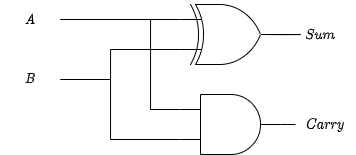
1-bit full adder
The full adder includes a carry in input.
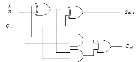
N-bit full adder
The n-bit full adder can be created by chaining 1-bit full adders.
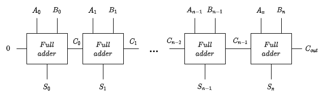
N-bit adder/subtractor
An adder/subtractor can be created by adding a control line, $Z$. When
the line is low, the second number is added to the first and when it's
high the second number is subtracted.
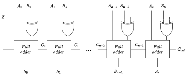
When $Z$ is high the circuit applies two's complement to the second number by inverting the bits using the XOR gates and adding 1 using the carry in. When $Z$ is low it works the same as the normal n-bit adder.
Active high and active low
Circuits can be either active high or active low. In an active high circuit a 1 is active and a 0 is inactive. In an active low circuit a 0 is active and a 1 is inactive.
Encoder and decoder
An encoder takes $n$ distinct inputs and maps them to a combination of $\log n$ outputs. The following shows an active-high 4 to 2 encoder and it's truth table.
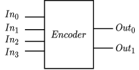
| $In_0$ | $In_1$ | $In_2$ | $In_3$ | $Out_0$ | $Out_1$ |
|---|---|---|---|---|---|
| 1 | 0 | 0 | 0 | 0 | 0 |
| 0 | 1 | 0 | 0 | 0 | 1 |
| 0 | 0 | 1 | 0 | 1 | 0 |
| 0 | 0 | 0 | 1 | 1 | 1 |
A decoder takes $n$ inputs and maps them to one of $2^n$ distinct outputs. The following shows an active-high 2 to 4 decoder and it's truth table.
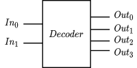
| $In_0$ | $In_1$ | $Out_0$ | $Out_1$ | $Out_2$ | $Out_3$ |
|---|---|---|---|---|---|
| 0 | 0 | 1 | 0 | 0 | 0 |
| 0 | 1 | 0 | 1 | 0 | 0 |
| 1 | 0 | 0 | 0 | 1 | 0 |
| 1 | 1 | 0 | 0 | 0 | 1 |
Encoders can be used to translate analogue signals into digital ones and decoders can be used for addressing memory locations in a processor.
Multiplexer and demultiplexer
A multiplexer (shortened to mux) takes $n$ inputs and $\log n$ switches to decide which input should be the output.
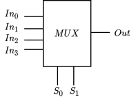
| $S_0$ | $S_1$ | $Out$ |
|---|---|---|
| 0 | 0 | $In_0$ |
| 0 | 1 | $In_1$ |
| 1 | 0 | $In_2$ |
| 1 | 1 | $In_3$ |
A demultiplexer (shortened to demux) does the opposite of a multiplexer.
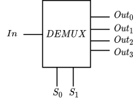
| $S_0$ | $S_1$ | $Out_0$ | $Out_1$ | $Out_2$ | $Out_3$ |
|---|---|---|---|---|---|
| 0 | 0 | $In$ | 0 | 0 | 0 |
| 0 | 1 | 0 | $In$ | 0 | 0 |
| 1 | 0 | 0 | 0 | $In$ | 0 |
| 1 | 1 | 0 | 0 | 0 | $In$ |
Multiplexers and demultiplexers can be used in communication systems. They allow multiple signals to be transmitted on a single cable, such as a telephone line. They are also used in other scenarios where inputs and outputs need to be switched between.
Sequential logic circuits
A logical circuit whose outputs are a logical function of it's inputs and it's current state. Unlike combinatorial logic circuits, these circuits have some element of memory.
Flip flops
A flip flop is the most basic memory circuit. It has two stable states (bistable) which allows it to store a single bit of data. The state can be changed by activating some control input. The circuit below shows an $\overline{SR}$ NAND latch.
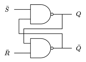
$\bar{S}$ and $\bar{R}$ are set and reset inputs respectively. The NAND latch is active low, hence the bars over the inputs. $Q$ and $\bar{Q}$ are the outputs and $\bar{Q}$ is the inverse of $Q$. Both inputs should never be active at the same time. The latch has the following truth table (remember it's active low):
| $S$ | $R$ | $Q$ | $\bar{Q}$ |
|---|---|---|---|
| 1 | 1 | No change | No change |
| 1 | 0 | 1 | 0 |
| 0 | 1 | 0 | 1 |
| 0 | 0 | Invalid | Invalid |
D-type latch
A D-type latch is created using the $\overline{SR}$ NAND latch. It has one data input and an enable line. The state will only be modified when the enable line is high. The design of the circuit prevents the invalid state because when the enable line is low both are high and if the enable line is high the negation ensures only one is ever low at a time. Note that the D-type latch is active high.
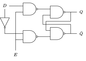
| $D$ | $E$ | $Q$ | $\bar{Q}$ |
|---|---|---|---|
| 0 | 0 | No change | No change |
| 1 | 0 | No change | No change |
| 0 | 1 | 0 | 1 |
| 1 | 1 | 1 | 0 |
The enable line is often connected to a clock. The state of the D-type is then changed on the rising edge of the clock (from 0 to 1). The D-type latch is often represented as below, where the $>$ input is the enable line/clock input.
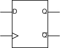
N-bit register
The n-bit register is made from multiple D-type latches. A register can have parallel or serial inputs and outputs. Parallel is all the bits at once, serial is one bit at a time. The register below is a parallel in/parallel out n-bit register.
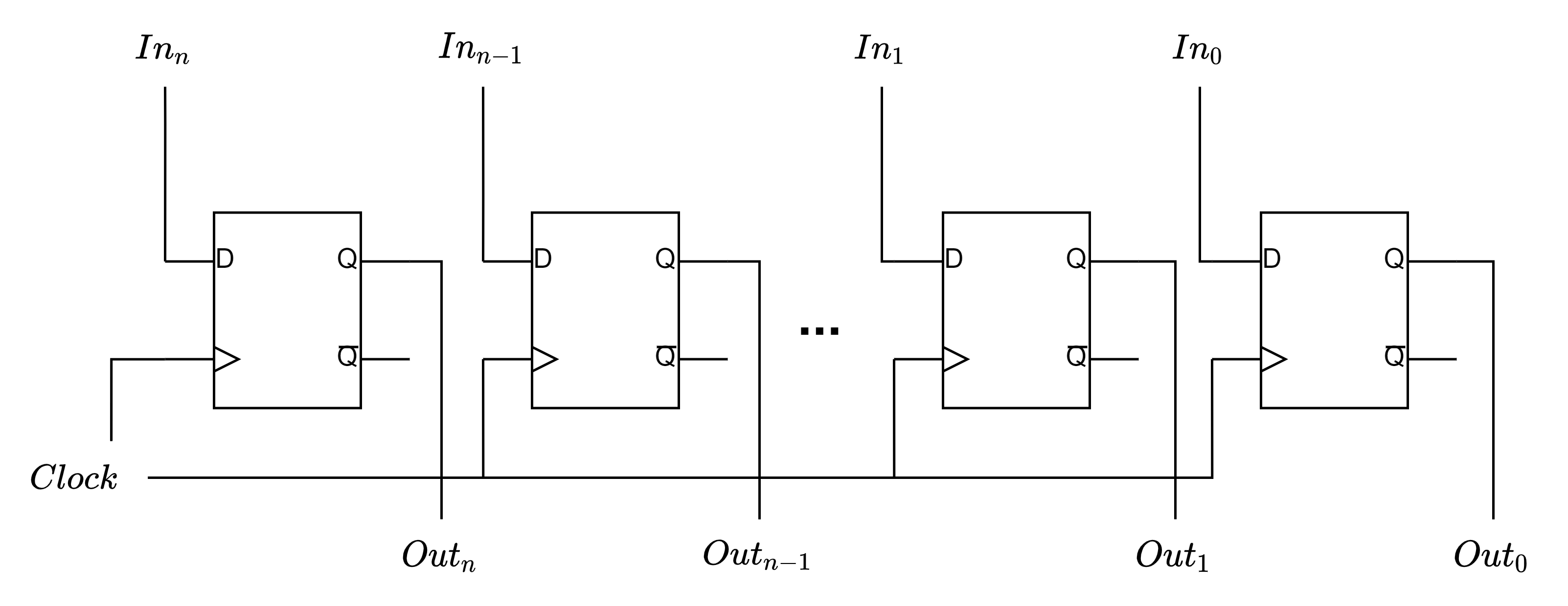
N-bit shift register
A shift register shifts it's contents every clock tick. The below register is a serial in/parallel out n-bit shift register.
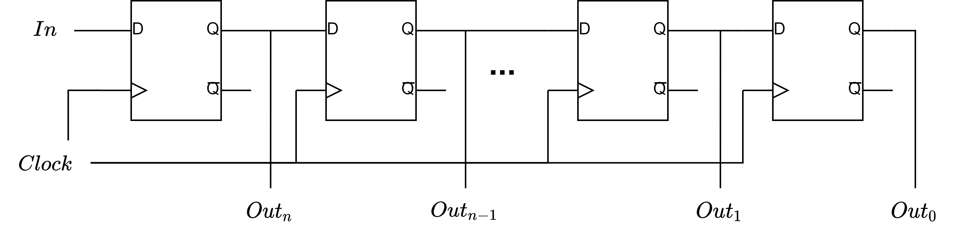
N-bit counter
The n-bit counter counts up in binary. The leftmost D-type is clocked as normal. Every D-type has it's input as it's inverted output. Each subsequent D-type is triggered on the falling edge of the previous D-type (represented by the circles on the clock input below).
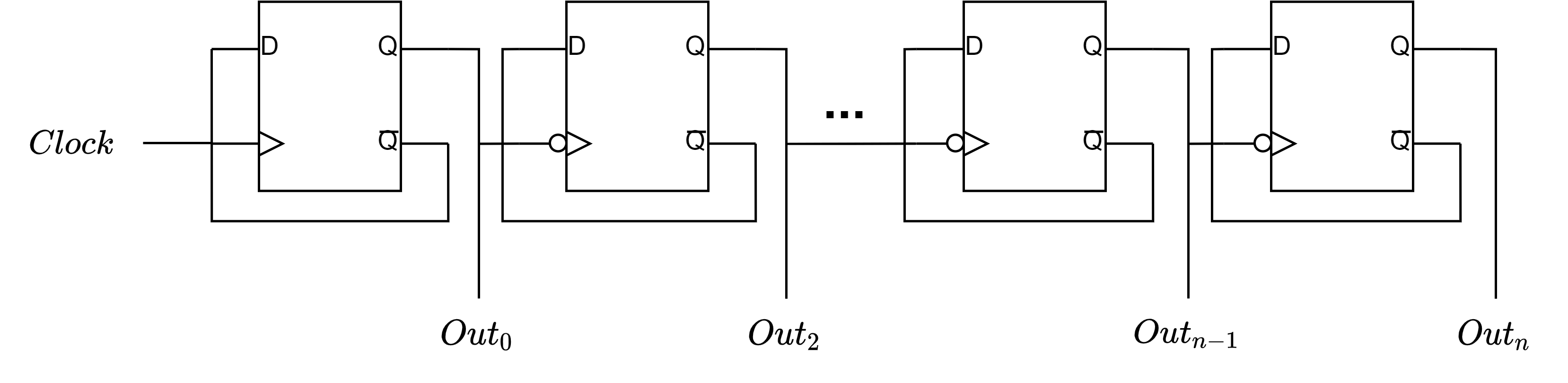
The n-bit counter works as follows:
Initial: The clock is low, the output of all D-types is 0.
Rising edge 1: The first D-type is clocked on the rising edge of the clock. $Out_0$ is now 1 because that was the value of $\bar{Q}$. The output has risen, so the second D-type is not clocked. Reading right to left, the output is now 00...0001, binary for 1.
Rising edge 2: The first D-type is clocked, it's input is $\bar{Q} = 0$, so the output is now 0. The output has fallen from 1 to 0, so the second D-type is now clocked. It's input is 1, so it's output is now 1. Reading right to left the output is now 00...0010, binary for 2.
Rising edge 3: The first D-type is clocked and is now 1. The output has risen so the second is not clocked. The overall output is now 00..0011, binary for 3.
Rising edge 4: The first D-type is clocked and is now 0. The output has fallen so the second D-type is clocked and is now 0. The second D-type output has fallen so the third D-type is clocked and is now 1. The overall output is now 00..0100, binary for 4.
This pattern will then repeat, counting up in binary.
Three state logic
Logic components considered so far have two states, 1 or 0. A 3-state buffer has an additional state, unconnected activated by the $\overline{Enable}$ line, which is active low.
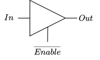
When $\overline{Enable}$ is high the buffer is unconnected, when it is low the input and output are connected. Three state buffers allow shared buses by allowing one data source on to the bus at once.
Physical implementations
Propagation delay
Propagation delay is the time taken for a logic gate to work, usually nanoseconds. This limits the speed at which logic circuits can work. Propagation delay can be reduced by making gates physically closer.
Integrated circuits
An integrated circuit is a collection of components on a single chip. These can be simple logic gates or programmable devices which allow larger circuits to be created. Programmable logic devices include the following:
-
Programmable Array Logic (PAL) - Programmable AND array and fixed OR array.
-
Programmable Logic Array (PLA) - Programmable AND and OR arrays.
-
Field Programmable Gate Array (FPGA) - Array of programmable logic blocks, which can be used for complex combinational functions or simple logic gates. FPGAs are usually reprogrammable.
Microprocessor fundamentals
CPU
The CPU controls and performs instructions. The CPU has a fetch-decode-execute cycle which continuously performs instructions.
The CPU consists of many components and registers.
-
Arithmetic logic unit - Performs mathematical and logical operations.
-
Control unit - Decodes instructions and handles execution.
-
Instruction register - Holds the most recent instruction
-
Memory address register - Holds the address of memory for reading or writing.
-
Memory data register - Holds the data retrieved from or to be written to memory.
Fetch-decode-execute cycle
-
Fetch - Copy address of next instruction from PC to MAR. The PC is incremented. Get the data at the location in the MAR and copy it into the MDR, then copy that to the IR.
-
Decode - The instruction in the IR is split into it's opcode and operand by the CU.
-
Execute - The CU sends the necessary signals to execute the instruction.
The instruction is then decoded into the opcode and operand, after which the CU sends the necessary signals to execute it.
Register transfer language
Register transfer language (RTL) is used to describe register operations. For example [IR] $\leftarrow$ [MDR] means the contents of the MDR are copied to the IR. [MS(...)] refers to the contents of main store at the address specified.
The fetch-decode execute cycle can be represented using RTL.
-
$[\text{MAR}] \leftarrow [\text{PC}]$
-
$[\text{PC}] \leftarrow [\text{PC}] + 1$
-
$[\text{MDR}] \leftarrow [\text{MS}([\text{MAR}])]$
-
$[\text{IR}] \leftarrow [\text{MDR}]$
-
$\text{CU} \leftarrow [\text{IR}]$
Assembly language
Assembly language is one level above machine code. It uses mnemonics which map closely to machine code instructions. Assembly code is converted into machine code by an assembler.
Assembly language has a variety of instructions including those for moving data, arithmetic, logic, branching and subroutines.
Addressing modes
Addressing modes are different ways of telling the processor where to find data. Addresses can be absolute, indirect or relative or may be a literal value.
Memory systems
Memory hierarchy
The memory hierarchy refers to the relative speed and cost per size of different memory technologies. Registers are the fastest memory as the are the closest to the CPU, but they are not suitable for mass storage. Cache is slower than registers but still close to the CPU and fast, but too expensive for mass storage. RAM is ideal for volatile storage of quite a lot of data needed by the CPU and isn't too expensive. Hard disks are slower to access but much cheaper for large amounts of storage.
Locality
Temporal locality - If a memory location is referenced it's likely the same location will be referenced again soon.
Spatial locality - If a memory location is referenced it's likely nearby memory locations will be accessed in the future. It has been shown that 90% of memory accesses are within 2 kilobytes of the previous PC position.
It's therefore a good idea to store data which is accessed frequently in memory as close to the CPU as possible and less frequently accessed data in slower, cheaper storage.
Cache memory
Cache memory is a small amount of memory between the RAM and CPU.
Cache hit and miss
It is much faster for the CPU to retrieve data from the cache than from RAM. If the data the CPU is looking for is in the cache then that is a cache hit and this is good as the data can be retrieved quickly. When the CPU needs data and it isn't in the cache that is a cache miss. The hit rate of the cache is given by the number of cache retrievals over the total number of retrievals.
There are several type of cache miss.
-
Compulsory - Misses that would occur regardless of cache size
-
Capacity - Misses that occur because the cache is not large enough
-
Conflict - Misses that occur due to inefficient cache organisation
-
Coherency - Misses that occur due to cache flushes in multiprocessor systems
Multilevel cache
Cache is often split into several levels between the CPU and RAM. Level 1 (L1) cache is the closest and therefore fastest but also smallest, then L2 cache which is slightly slower but larger and L3 cache, further but larger.
Memory organisation
Semiconductor memory
Semiconductor memory is the most common form of main store, more commonly known as RAM. There are two types, static RAM and dynamic RAM. SRAM uses a flip-flop for each bit whereas DRAM uses capacitors. Both types are volatile. DRAM capacitors can leak charge so they need refreshing which incurs a one-off overhead but DRAM has larger capacity and is cheaper to produce so is often used for main memory. SRAM is faster but more expensive and is often used for cache.
Memory organisation
The basic memory element is a memory cell. It has two states, 0 or 1 and is capable of being written or read.
It is important to organise memory efficiently to reduce space and access time. Memory is accessed by row and column and it's important to choose the row/column sizes to reduce the number of addressing components.
Error correction
Errors can occur in a system or between systems. Noise is unwanted information which can lead to errors. It is caused by the physical properties of devices, such as heat and alignment of magnetic fields.
Parity bits
Errors can be detected through the use of a parity bit. This can be used to check if a message has been altered between the sender and receiver. There are two types of parity system - even and odd. In both systems the parity bit is set such that the total number of logical 1s is made to be either even or odd. If the message is invalid then the receiver can request retransmission.
Checksums
Parity bits are vulnerable to burst errors, where an error occurs for a short amount of time and all data sent will be erroneous. Instead, a checksum can be used which is computed from all of the data sent. Then if there is a burst error which affects a lot of the data it is still detected.
Error correcting codes
Error correcting codes use parity bit with checksums for even better error detection. They also allow for single error correction because the result from one check can be used to correct the errors in another.
IO mechanisms
Memory mapped IO
Memory mapped IO makes use of the same address bus for memory and IO devices. Memory on IO devices is mapped to address values and the CPU can then use them as normal. This is a simple approach and doesn't require much modification to the CPU but some amount of address space has to be reserved, which isn't ideal for processors with smaller word sizes.
Polling
Most IO devices are slower than the CPU so there needs to be a way to check when the IO devices are ready. One approach is polling. The CPU can poll the IO devices to see whether they are ready to give or receive data. There are two types of polling, busy-wait and interleaved. The former is a loop of checking the status until the device is ready, doing nothing in between. This is ideal for systems which need to respond quickly to IO devices but wastes CPU power and processing time for the average device. Interleaved polling allows the processor to do other task while it waits, but this can mean a delayed response to IO devices. Polling is a simple technique which doesn't need complex hardware or software and is ideal for some applications.
Handshaking
Handshaking can be used to synchronise the CPU and IO devices. The CPU can tell the IO device it's sent valid data and the IO device can tell the CPU it's ready.
Interrupts
Interrupts interrupt the current execution state of the processor with an interrupt service routine (ISR). The current state of the registers is pushed to the stack, then the ISR is executed and then the original state is restored from the stack. There are two types of interrupt - interrupt request (IRQ) and non-maskable interrupt (NMI). It is possible to ignore an IRQ but no and NMI. Interrupts allow a fast response and don't waste CPU time and power, but data transfer is still handled by the CPU creating a bottleneck and the hardware and software needed are more complex.
Direct memory access
Direct memory access (DMA) is used when large amounts of data need to be transferred quickly. It uses a DMA controller (DMAC) to take control of the system buses. It can then efficiently transfer data from IO devices to storage. The DMAC is optimised for data transfer and can be more than 10 times faster than CPU IO.
Modes of operation
-
Cycle stealing - The DMAC uses the system buses when they're not being used by the CPU
-
Burst mode - The DMAC takes control of the system buses for a fixed time unless the CPU receives a higher priority interrupt.
Organisation
-
Single bus detached - DMAC, IO, memory and processor share the same system buses. This is more straightforward but less efficient.
-
IO Bus - The DMAC uses the system buses and also has a dedicated IO bus which is connected to IO devices.
Processor architecture
Organisation and architecture
Organisation and architecture involves the structure and properties of a computer system, but organisation is from the perspective of a hardware engineer and architecture from a software engineer.
Micro and macro instructions
Mnemonic assembly instructions are macro operations which consist of smaller, register-level operations called micro instructions. The CU knows control signals to send for each micro operations for a given macro instruction. For example, the ADD instruction has several micro instructions for copying registers to the ALU, setting control signals and copying the result.
Control unit design
The control unit is responsible for taking an instruction and sending the necessary signals to execute it. There are two approaches to CU design, hardwired and microprogrammed.
A hardwired (also called random logic) CU is a combinatorial logic circuit. This is a fast method but is complex and difficult to modify. It is more commonly used for RISC processors.
A microprogrammed CU functions like a very basic processor. Each machine instruction is turned into a sequence of microinstructions which are then executed. This is much more easy to design and implement and is also easier to reprogram, but is slower than hardwired CUs. It is more commonly used for CISC processors.
RISC and CISC
RISC and CISC are two types of instruction set. RISC uses fewer, more commonly used instructions whereas CISC has far more instructions which might not be used as often. RISC programs are usually more verbose but more efficient, whereas CISC programs are shorter but slower.
CS139 - Web Development Technologies
These notes do not cover learning Python or JavaScript and only briefly cover Flask and Jinja.
HTML
Introduction
HTML (Hyper Text Markup Language) is the markup language used for the structure and content of a web page. HTML consists of elements which are defined using tags. An example of a basic HTML page:
<!DOCTYPE html>
<html>
  <head>
    <meta charset="utf-8">
    <title>"Welcome</title>
  </head>
  <body>
    <h1 id = "title" class = "green-text">Welcome to our website</h1>
    <p>This text is <strong>very</strong> important.
    <img src = "images/logo.png" alt = "Our logo"/>
  </body>
</html>
The first line is the doctype declaration. This tells the browser this is a HTML5 document.
The <html> tag surrounds the entire contents of the page.
The <head> section contains metadata about the web page such as the
title, character set, author, keywords and links to other files.
The <body> contains all of the visible content on the page.
<h1> is the largest heading tag. There are 6 levels of heading, <h1>
to <h6>. It has both an id and class. An id needs to be a unique
identifier for this element but a class can be used for multiple
elements.
Tags can be nested, like the <strong> tag inside the p. This will
make only the word "very" bold.
<img> has just attributes and no content. The alt text is good for
accessibility as it provides a description of an image for screen
readers.
Relationships
h1 is the child of body and body is the parent of h1. h1, p
and img are siblings because they all have the same parent. h1, p,
strong and img are descendants of body. html is an ancestor of
strong.
Lists
There are two types of list, ordered and unordered. An example of an ordered list:
<ol>
  <li>Grate 50g of cheese</li>
  <li>Add 2 eggs and combine</li>
  <li>Boil a large saucepan of water</li>
</ol>
<li> means list item. Use <ul> instead of <ol> for unordered
lists.
Character entities
Character entities can be used for characters like > which would
otherwise be mistaken for HTML or for symbols like . For example, > is
> and is ©.
Tables
Tables are defined using the <table> tag. An example table:
<table>
  <thead>
    <tr>
      <th>Name</th>
      <th>Age</th>
      <th>Nationality</th>
    </tr>
  </thead>
  <tbody>
    <tr>
      <td>Maria</td>
      <td>44</td>
      <td>Belgian</td>
    </tr>
    <tr>
      <td>Barry</td>
      <td>63</td>
      <td>British</td>
    </tr>
  </tbody>
</table>
The table consists of a head (thead) and body (tbody). Each row is
contained within a tr (table row) and each cell is either th (table
header) or td (table data).
To make a table cell take up multiple rows/columns, use the rowspan
and colspan attributes respectively.
Forms
HTML forms can be used to send data to the server.
<form action="/login" method="POST">
  <label for="usrnm">Username:</label>
  <input type="text" name="username" id="usrnm" required>
  <label for="pswd">Password:</label>
  <input type="password" name="password" id="pswd" required>
  <input type="submit" value="Log in">
</form>
Forms consist of an action, a method and fields. The action tells the
browser where to send the form data and the method says how. The method
is usually GET or POST. GET sends the data as URL parameters and POST
sends the data in the request body. The contents of the form consists of
label and input elements. Labels just describe what the input is
asking for. The for attribute corresponds to the id attribute of the
input. There are many different types of input, the most common being
text, email, password and submit. The required attribute tells the
browser to make sure that field is filled in before submitting the form.
Semantic HTML and accessibility
HTML is semantic if it gives meaning to it's contents. For example,
using tags like <main>, <article>, <aside>, <header> and
<footer> is much more descriptive than just using <div>. This
improves SEO (search engine optimisation) and makes the site more
accessible.
Tables should only be used for data, not layout as otherwise this can cause issues for screen readers. Using labels on forms and alt text for images helps to make sites more accessible.
CSS
CSS (Cascading Style Sheets) are used to define the styles for an HTML
page. Styles can either be included inline, in a style tag or in an
external .css file.
Inline:
<p style = "color:red;">Red text</p>
style tag:
<head>
  <style>
    p{
      color: red;
    }
  </style>
</head>
External file:
<head>
  <link rel = "stylesheet" type = "text/css" href = "style.css"/>
</head>
File style.css:
p{
  color: red;
}
CSS rules consist of a selector and one or more declarations. A
declaration consists of a property and it's value. In the examples
above, the selector is p (all paragraph elements) and the declaration
has property color (the foreground text colour) with value red.
HTML classes and IDs can be used to style individual elements or groups
of elements. The selector for a class is .classname and the selector
for an id is #idname.
Attribute selectors
Attribute selectors can be used to select elements with specific
attributes. For example,
input[type="password"] will apply the style to all input elements
where the type attribute is password.
Pseudo-classes
Pseudo-classes are an additional part to a selector which sets the style
for a particular state. For example, button:hover selects buttons
which are being hovered over. a:visited selects links which have
already been clicked. There are many other pseudo-classes including
selectors for the first or nth child of an element.
Pseudo-elements
Pseudo-elements are an additional part to a selector which style a
specific part of the element (as opposed to a specific state for
pseudo-classes). p::first-line can be used to style the first line of
a paragraph.
Other selectors
div p selects p elements which are descendents of div elements.
div>p selects p elements which are children of div elements.
div~p selects p elements which are siblings or descendents of
div.
div+p selects p only if it appears immediately after div and they
have the same parent.
The box model, block and inline
The box model represents the content, padding, margin and border of an
element and determines how it appears on the page.
Block level elements end with a new line. These include <h1>, lists
and tables.
Inline elements are in line with other elements. These include <a> and
<img>.
Media queries
Media queries allow for responsive web design by adapting styles based
on the size of the user's screen. The basic syntax is
@media mediatype and mediafeature. In the following example the
background will be green for screens above 800px wide and red for
screens narrower than 800px but wider than 400px.
@media screen and (min-width: 400px) {
  body {
    background-color: red;
  }
}

@media screen and (min-width: 800px) {
  body {
    background-color: green;
  }
}
screen is the media type for any screen, but there is also print for
printed documents and speech for screen readers. As well as
min-width there is max-width, min-height and max-height as well
as resolution and device orientation. Different queries can be combined
with and and or. For example, this media query will match devices
whose width is between 320px and 480px.
@media only screen and (min-width: 320px) and (max-width: 480px) {
  body {
    background-color: blue;
  }
}
Python and Flask
Python is high-level general purpose programming language. It's easy to learn and there are a lot of good resources available online. These notes do not aim to teach Python and only provide a brief overview of Flask.
Virtual environments
When doing a Python project, it's a good idea to contain it within a
virtual environment. This allows you to install a library for one
project without installing it everywhere. A good guide is
https://python.land/virtual-environments/virtualenv. In Python 3.4 and
above, you create the virtual environment by running
python -m venv [directory]. Usually you want the virtual environment
in your current directory, so run python -m venv venv. This will
create a virtual environment in a directory called venv.
To activate the virtual environment, run venv.bat on Windows or
source venv/bin/activate on Linux or MacOS. You have to activate the
virtual environment every time before you can use it. Once it's
activated anything you install will only be installed inside it. You can
then deactivate it by running deactivate.
Serialisation
Serialisation in Python is done using the pickle module.
>>> capitals = {'Greenland': 'Nuuk',
                'Luxembourg': 'Luxembourg',
                'Trinidad and Tobago': 'Port of Spain',
                'Romania': 'Bucharest'}
>>> serialised = pickle.dumps(capitals)
>>> print(serialised)
b'\x80\x04\x95c\x00\x00\x00\x00\x00\x00\x00}\x94(\x8c\tGreenland\x94\x8c\x04Nuuk\x94\x8c\nLuxembourg\x94h\x03\x8c\x13Trinidad and Tobago\x94\x8c\rPort of Spain\x94\x8c\x07Romania\x94\x8c\tBucharest\x94u.'
>>> loaded = pickle.loads(serialised)
>>> loaded == capitals
True
Data can be serialised to bytes (binary which anything can store) and then deserialised back into a Python object. This is useful for databases as they can't store Python objects but they can store binary.
A more widely used form of serialisation (not Python specific) is JSON
(Javascript Object Notation). It is natively supported in Javascript and
is often used for sending data between a client and server but is also
widely supported by many programming languages and systems, making it an
ideal language agnostic method of transferring data. In Python the
json module provides loads and dumps methods for converting
between JSON and Python dictionaries.
Flask
Flask is a web micro-framework written in Python. It is not installed by
default so you need to install it with pip install flask. It provides
a way to respond to requests using routes and send responses. It makes
uses of Jinja for templates and has extensions for interfacing with
databases, authentication and forms. A basic Flask app is shown below:
from flask import Flask

app = Flask(__name__)

@app.route("/")
def index():
    return "Website is working"
This app can be run with flask run from the command line.
The first line imports Flask and the second creates the Flask app. The
__name__ helps Flask work out which folder it's in.
The @app.route is called a decorator and it says that the function
defined below is how Flask should respond to a request for /, which is
the root of your website. The function index is called whenever this
request is made and the message it returns is sent as a response.
Basic forms
Suppose we have the form from the last section in
a file called index.html in a directory called templates and the
following Python file in the current directory:
from flask import Flask, request, render_template, redirect

app = Flask(__name__)

@app.route("/")
def index():
    return render_template("index.html")

@app.route("/login", methods = ["POST"])
def login():
    print(request.form["username"] + "\n" + request.form["password"])
    return redirect("/")
Flask can get request parameters using the request object. You have to
import this from flask. request.form allows you to access form
parameters, request.method gives you the request method (usually GET
or POST) and request.args.get(...) allows you to access the GET
parameters. In the example above the username and password sent will be
printed out. The "username" and "password" correspond to the name
attributes of the inputs in the form.
Security
Passwords can be hashed using the Werkzeug security module. Generate a
hash using
generate_password_hash(password) and check it using
check_password_hash(hash, password).
Jinja
Flask templates use the Jinja template engine to produce HTML
dynamically. Templates are stored in the templates directory. A Jinja
template is just a normal HTML file but some parts are placeholders
instead.
Example template:
<!DOCTYPE html>
<html>
    <head>
        <title>{{ title }}</title>
    </head>
    <body>
        {% if weekday %}
          <p>It's {{ dayOfWeek }}. You get 10% off!</p>
        {% else %}
          <p>Come back any time in the week to get 10% off.</p>
        {% endif %}
    </body>
</html>
The double braces are placeholders for expressions and the lines
beginning with % are statements. For example, title will be replaced
with the value of the variable title, which is passed to the template
using render_template.
The if statement causes the template to render differently depending on
whether it's a weekday or not. There are also % for % statements for
iteration.
This template would be returned by a Flask route using
return render_template("index.html", title = "Special offer", weekday = True, dayOfWeek = "Wednesday")
It is also possible to include files in other templates using
% include:
<main>
  ...
</main>
{% include "footer.html" %}
</body>
Databases and SQL
Databases are used to store data. SQLite is a simple database engine which uses SQL for queries. SQL (Structured Query Language) is a language used to interface with databases. A database consists of tables, which consist of columns called fields and rows called records. Each column has a fixed data type and each row is a single entry into the database. For example, users could be a table, username could be a field with type text and each user would have a record.
Data types
There are 4 data types in SQLite: text, integer, real and blob (binary data).
Basic operations
Create table:
CREATE TABLE users(
  id INTEGER PRIMARY KEY,
  username TEXT UNIQUE NOT NULL,
  password TEXT NOT NULL
);
Note: A column with type INTEGER PRIMARY KEY will auto-increment.
Delete table:
DROP TABLE users;
Insert record:
INSERT INTO users (username, password) VALUES ('bob', '513e35...0e7252');
Select record:
SELECT username, password FROM users WHERE id = 1;
Update record:
UPDATE users SET username = 'steve' WHERE id = 1;
Delete record:
DELETE FROM users WHERE id = 1;
Additional parts
ORDER BY column - Ascending order the results by column.
ORDER BY column DESC - Descending order the results by column.
LIMIT n - Give the first $n$ results.
Relationships
It is possible to create relationships between tables using foreign keys. This is a field in one table which refers to the primary key in another.
SQLAlchemy
SQLAlchemy is a Python ORM (Object-Relational Mapping) for working with
databases as objects in Python instead of raw SQL. There is a wrapper
for Flask, flask-sqlalchemy, which can be used to work with databases
in Flask applications.
Integrating into a Flask app
To add a database to an app, do the following:
from flask import Flask
from flask_sqlalchemy import SQLAlchemy

app = Flask(__name__)
app.config["SQLALCHEMY_DATABASE_URI"] = "sqlite:///dbname.db"
app.config["SQLALCHEMY_TRACK_MODIFICATIONS"] = False
db = SQLAlchemy(app)
The app is now linked to the database but needs models to work with it.
Executing raw SQL
It is still possible to execute raw SQL queries through SQLAlchemy using
db.session.execute.
from sqlalchemy import text
db.session.execute(sqlalchemy.text("SELECT * FROM users WHERE id = :val"), {"val": 1})
Database operations
Using the same examples as for raw SQL, the models file would be
from app import db

class User(db.Model):
    id = db.Column(db.Integer, primary_key = True)
    username = db.Column(db.Text, nullable = False, unique = True)
    password = db.Column(db.Text, nullable = False)
This can then be created by running db.create_all().
A record can be inserted by creating an instance of the model class,
then using db.session.add:
new_user = User(username = "bob", password = "513e35...0e7252")
db.session.add(new_user)
db.session.commit()
For changes to be saved, you need to commit them using
db.session.commit().
There are two ways to get a record from the database. The first is using
db.session.query:
db.session.query(User).get(1). This gets the User object with id 1.
The other, simpler method is using User.query.get(1) which returns the
same thing.
To get records by something other than id you can use filter_by.
User.query.filter_by(name = "bob") is equivalent to
SELECT * FROM users WHERE name = ’bob’. This will return a list of
results even if there is only one result or None if there are none.
User.query.filter_by(name = "bob").first() will return the first
record that matches and User.query.filter_by(name = "bob").all() will
return all matching records.
To get all records in a table use User.query.all()
A record can be updated by getting it, then modifying it's attributes and commiting.
user = User.query.get(1)
user.name = "steve"
db.session.commit()
A record can be deleted by getting it and using db.session.delete.
user = User.query.get(1)
db.session.delete(user)
db.session.commit()
Relationships
Suppose we have two tables User and Post as follows:
from app import db

class User(db.Model):
  id = db.Column(db.Integer, primary_key = True)
  username = db.Column(db.Text, nullable = False, unique = True)
  password = db.Column(db.Text, nullable = False)

class Post(db.Model):
  id = db.Column(db.Integer, primary_key = True)
  title = db.Column(db.Text, nullable = False)
  content = db.Column(db.Text, nullable = False)
To create a relationship between these tables we can use db.ForeignKey
and db.relationship.
from app import db

class User(db.Model):
  id = db.Column(db.Integer, primary_key = True)
  username = db.Column(db.Text, nullable = False, unique = True)
  password = db.Column(db.Text, nullable = False)
  posts = db.relationship("post", backref = "author", lazy = "dynamic")

class Post(db.Model):
  id = db.Column(db.Integer, primary_key = True)
  title = db.Column(db.Text, nullable = False)
  content = db.Column(db.Text, nullable = False)
  author_id = db.Column(db.Integer, db.ForeignKey("user.id"))
Now Post has a column containing the author's id which is marked as a
foreign key which is the id field of the user table.
The relationship gives User a new attribute posts which is a list of
all of the posts whose author_ids are the user's. The backref means
that Post now has an author attribute so you can easily get it's
author's User object. lazy = dynamic just means that a query object
is returned instead of a list of objects so you can then call something
like filter_by on it.
Protocols
A protocol is a shared standard set of rules which allows two parties to communicate.
Internet protocol suite
The main protocols used for the internet are called the internet protocol suite. This consists of 4 layers, application, transport, internet and link.
The application layer is made up of protocols such as HTTP/HTTPS (Hyper Text Transfer Protocol (Secure)), DNS (Domain Name System), FTP (File Transfer Protocol) and SMTP (Simple Mail Transfer Protocol) as well as many others. These protocols are used by applications to standardise communications. These work with the transport layer to send and receive data.
The transport layer consists of protocols like TCP and UDP (User Datagram Protocol). These protocols ensure the successful transfer of packets.
The internet layer uses IP. This is responsible for addressing and routing packets between networks. There are two main versions, IPv4 and IPv6. The former uses 32 bits for an address for a possible 4,294,967,296 addresses. This was not enough, so IPv6 was introduced and uses 128 bit IP addresses giving $3.4 \times 10^{38}$ total addresses.
The link layer works on the lowest level transmitting bits through a local network.
Network address translation
NAT involves modifying the network address of packets when they're being routed through a device. This allows multiple computers on a local network to use one public IP address. When the router receives a packet it determines which local machine to route it to.
DNS
DNS (Domain Name System) translates human readable domain names into IP addresses. A domain name consists of multiple levels. Top level domain domains (TLDs) include .com, .co.uk and .org, then second level domains are the domain names people can register. Any lower levels are known as subdomains.
DNS resolution
The client sends a query to a DNS recursor. The DNS recursor queries the root nameserver, which points to the TLD nameserver (.com nameserver for example) which will then point to the authoritative nameserver (example.com nameserver for example) which will provide the desired IP address which is then sent back to the client. Often the recursor will cache records for faster lookups.
Uniform Resource Locators
A URL (Uniform Resource Locator) is a reference to something on the
internet. It consists of a scheme, such as HTTPS or FTP, a host such as
a domain name, a path and optional query and fragment. In
https://www.example.com/example?page=12#about, HTTPS is the scheme,
www.example.com is the host, ?page=12 is the
query and #about is the fragment.
HTTP
HTTP is the protocol responsible for web requests and responses.
The two most common types of HTTP request are GET and POST. A GET
request is used to request a resource. A POST request is used to send
data to a server. HTTP requests consist of the method (GET/POST), the
path, the version of the protocol (usually HTTP/1.1) and the headers.
HTTPS responses consist of the protocol version, status code, status message, headers and optional content.
Headers contain information about a request or response such as the content length, type, language or encoding, the date it was sent and many others.
Some status codes and messages:
| Code | Message |
|---|---|
| 200 | OK |
| 301 | Moved permanently |
| 302 | Found |
| 304 | Not modified |
| 400 | Bad request |
| 403 | Forbidden |
| 404 | Not found |
| 405 | Method not allowed |
| 414 | Request URI too long |
| 418 | I'm a teapot |
| 500 | Internal server error |
| 503 | Service unavailable |
HTTPS
HTTPS provides a secure connection over SSL/TLS (Secure Socket Layer/Transport Layer Security). Data is encrypted between the client and server which is ideal for sending sensitive information as anyone listening in on a connection can't understand what's being sent. The client sends the server it's preferred SSL/TLS options and the server uses the most secure option supported by both. Then the server sends it's certificate which the client can verify is signed by a trusted certificate authority. The client can now send the server an encrypted key that it can use to encrypt their traffic.
Statelessness
HTTP is a stateless protocol. This means there is no link between two different requests from the same connection. This can be resolved by using query strings, cookies and sessions. The query string in a GET request can be used to send additional data to the server. Cookies are sent between the server and client in the headers. Cookies expire after a given time. Cookies can be used to provide sessions. The cookie will hold an identifier which the server can relate to some stored data about the client.
POST redirect
If the user sends a POST request, then refreshes the browser the browser will send the last request (the POST request) again. This can cause problems if the POST request was a payment authorisation, for example. To avoid this the server must redirect the user after a POST request. This redirect causes a GET request so when they refresh the GET request is sent again, not the POST request.
Security
Passwords
Passwords should never be stored as plain text. If the database was breached then the attackers have instant access to every account and could even use the stolen credentials to try and gain access to accounts on other websites. A hash function is a one-way function which always gives the same, fixed-length output for the same input. Common hashing algorithms include MD5, SHA-256 and bcrypt. Hashing is used to make the password infeasible to recover for attackers. Hashing alone is not sufficient though, as it is easy to precompute a table of common passwords and their hashes. Adding a salt to the end of the password, then hashing provides better security. When the user registers an account the password is salted and hashed and then the hash and salt are stored in the database. When the user signs in the salted hash of their given password is compared to the stored hash. If they match then the user has given the right password and can be allowed access.
SQL injection
Poorly handled user input can lead to SQL injection. This is where the
user sends text specially formatted to trick the server into running SQL
it didn't intent to.
Consider the following:
cursor.execute("SELECT * FROM records WHERE firstName = '" + name + "'")
If the user input their name as name' OR 1=1;-- then all the records would
be returned. If the user input name'; DROP TABLE records;-- and the database
allowed multiple queries then the records table would be deleted.
To prevent SQL injection it is important to parameterise SQL queries. The method for this varies by language and database but it ensures parameters are not interpreted as SQL and executed. SQLAlchemy is designed to prevent SQL injection so it is not as much of a concern when using it.
GET requests and sensitive data
GET requests should not be used to send sensitive data. GET parameters are visible in the address bar, but also visible to anyone listening to the connection, the routers, servers and logs even when using HTTPS because the URL isn't encrypted. This is not safe and POST request must always be used for sending sensitive data.
Session Hijacking
Session hijacking involves the exploitation of session cookies. Session sniffing involves listening to unencrypted traffic, intercepting cookies and then using then to impersonate a user. Session fixing involves tricking the user into logging in using a session ID known to the attacker. The attacker can then use this session ID and the server allows them access.
Cross site scripting
Cross Site Scripting (XSS) is a technique which allows an attacker to inject content into a web page. This is caused by poor input sanitisation. For example, if the user's query string was inserted directly into the web page, then HTML could be included in the query string to inject anything in to the page. If an unsuspecting user received an XSS login link and clicked it, the attacker could then inject their own form into the legitimate page and steal credentials, even though to the user the page seems legitimate. It is also possible to steal session cookies using this method, which can be used for session hijacking. To avoid XSS attacks, input should be sanitised and output should be escaped. Jinja does this by default.
Directory traversal
A user may request a file outside of the web server directory using a
path like ../../../etc/shadow. This can be prevented by configuring
the web server to only allow access to files within the web server
directory and using the secure_filename function in Flask.
JavaScript
JavaScript is an interpreted language often used on the client side. It
can be used to modify the content of a page, respond to events and make
requests. It is also useful for client side form validation. This can
decrease server load by not sending invalid requests, but data must be
validated on the server as well because client side validation is very
easy to bypass. Javascript is included in HTML using <script> tags
either inline or externally.
<!-- Inline -->
<script type = "text/javascript">
  window.alert("Inline Javascript");
</script>
<!-- External -->
<script type = "text/javascript" src = "scripts/external.js"></script>
Like Python there are plenty of resources to learn JavaScript.
Document Object Model
The Document Object Model (DOM) is a tree of the HTML elements in a page. JavaScript can access the DOM to make changes to the page. Elements can be accessed by their id, tag name and class. Any property of the element can then be modified using JavaScript, such as the style or text.
Events
Events are created in response to user actions with a page. Events can
be triggered by the page loading, the user clicking something, a
keypress or hovering over an element. To respond to an event you add a
handler function using addEventListener.
Event bubbling
Event bubbling is a feature of JavaScript where when an event is occurs,
it first checks if the element it happened to has any handlers, then if
it's parent has any, then it's grandparent all the way up to the top.
The events are said to bubble up from the deepest nested element to it's
parents. To stop bubbling, use event.stopPropagation.
JQuery
JQuery is a JavaScript library which simplifies DOM interactions and asynchronous requests.
AJAX
AJAX, which stands for Asynchronous JavaScript And XML, is a technique
which allows asynchronously updating the page without reloading.
Requests are sent asynchronously (in the background) so the user can do
other things whilst the request is being served. Whilst data can be
returned as XML, it is more common to use JSON now. XML (eXtensible
Markup Language) is markup language for storing data using HTML-like
arbitrary tags. In JavaScript, AJAX requests are sent using
XMLHTTPRequest objects. JQuery provides the much simpler $.ajax.
Usability and accessibility
Usability
Usability refers to the ease of use of a website for users. Usability can be achieved by improving ease of control, consistency, flexibility and efficiency of use. Quality documentation also helps make a system more usable as users understand what to do.
Accessibility
Accessibility involves making your website usable by people of all abilities and impairments. Websites should conform to WCAG (Web Content Accessibility Guidelines) and should use semantic HTML, appropriate layouts and alternative text for visual elements. Users may be using assistive technologies such as screen readers, magnification or Braille displays and websites should be compatible with them.
WCAG 2.1
WCAG 2.1 defines 4 accessibility principles.
-
Perceivable - Information and user interface components must be presentable to users in ways they can perceive.
-
Operable - User interface components and navigation must be operable.
-
Understandable - Information and the operation of user interface must be understandable.
-
Robust - Content must be robust enough that it can be interpreted reliably by a wide variety of user agents, including assistive technologies.
CS140 - Computer Security
These notes briefly cover everything in CS140.
Introduction
-
There is no such thing as absolute computer security
-
Theory is not the same as practice
CIA triangle
The CIA triangle states three key principles to consider in any secure system.
-
Confidentiality - No unauthorised disclosure
-
Integrity - No unauthorised change
-
Availability - Users who should be able to access something are able to
Terminology
-
Worm/virus - Self-replicating program which spreads across a network
-
DOS - Denial of Service, when a service is overwhelmed by a abnormally high volume of traffic
-
Social engineering - Exploiting a person to access a system
-
Asset - Anything of value which needs to be protected, such as a database, device or reputation
-
Vulnerability - A flaw in the design, implementation, operation or management of a system which can be exploited, such as weak passwords or a bug in a program
-
Threat - The potential for a security violation which occurs when an attacker has capability and intention
-
Risk - The expected loss given the threat, vulnerability and result
-
Attack - an assault on security from actioning a threat
-
Countermeasure - An action which prevents vulnerabilities, attacks or lessens their effects
Authentication
Passwords
Password strength and entropy
A longer password using a larger character set will be more secure. The number of possibilities is given by $p = w^l$, where $w$ is the size of the character set and $l$ is the length.
The number of possibilities can be very large, so a logarithmic scale is used to quantify strength. The entropy of a password is given by $x = \log_2 w^l$ or equivalently $l\log_2 w$. Entropy gives the theoretical uncertainty of a password, but in reality people are likely to use common words or numbers.
Hashing and salting
Passwords must never be stored as plain text. They should instead be hashed. Hash functions are one-way functions which return the same fixed length output for a given input. When the user enters a password, the hash can be compared to the stored hash. If they are the same the password is correct.
Salting a password before hashing it gives additional protection against lookup attacks as it will change the hash of the password. A salt is just some random data which is appended or prepended to the password before it is hashed. The salt is then stored alongside the hash so when the user enters a password, the salt can be added before comparing the hash.
Biometric authentication
Biometric authentication makes use of unique biological features, such as fingerprints or irises. This is ideal as only the intended user has the correct biological features, but it is susceptible to false positives.
Password cracking
Brute force attack
Try every possible input combination. Very inefficient.
Dictionary attacks
Use a list of common words or phrases which people are likely to use as passwords. Simple and usually effective.
Lookup tables
Pre-calculate the hash of many potential passwords, then look up an unknown hash to get the original password. Time efficient as hash tables have fast access and hashes only have to be calculated once. Space inefficient as a large number of password/hash pairs have to be stored.
Reverse lookup tables
Like a lookup table, but makes use of a hash chain. The hash chain is computed using a reduction function which maps hash values back into password values. The hash function and reduction function are applied a set number of times and only the first and last passwords are stored together.
To perform a lookup, apply the reduction and hash functions until a password matching an end password in the table is found. Then, take the start password and create the hash chain up until that point. The value before the hash being looked up is the desired password.
Reverse lookup tables are more efficient than simple lookup tables, but are susceptible to hash chain collisions, where two chains contain the same sub-chain at some point. This is redundant data and wastes space.
Rainbow tables
The rainbow table is designed to reduce chain collision by using different reduction functions for each reduction.
Public-key cryptography
Public-key cryptography makes use of two keys - a public key which can be shared freely and a private key which only its owner should have access to. The private key can be used to encrypt and decrypt messages, but the public key can only be used to encrypt.
Modular arithmetic
Public-key cryptography makes uses of the properties of modular arithmetic to encrypt and decrypt data using two keys.
There are several rules for working with modular arithmetic: $$ \begin{aligned} (A + B) \mathop{\mathrm{mod}}n &\equiv ((A \mathop{\mathrm{mod}}n)+B) \mathop{\mathrm{mod}}n\\ (A+B) \mathop{\mathrm{mod}}n &\equiv ((A \mathop{\mathrm{mod}}n)+(B \mathop{\mathrm{mod}}n)) \mathop{\mathrm{mod}}n\\ (A \times B) \mathop{\mathrm{mod}}n &\equiv ((A \mathop{\mathrm{mod}}n) \times B) \mathop{\mathrm{mod}}n\\ (A \times B) \mathop{\mathrm{mod}}n &\equiv ((A \mathop{\mathrm{mod}}n) \times (B \mathop{\mathrm{mod}}n)) \mathop{\mathrm{mod}}n\\ x^{A \times B} \mathop{\mathrm{mod}}n &\equiv (x^A \mathop{\mathrm{mod}}n)^B \mathop{\mathrm{mod}}n\\ (x^A \mathop{\mathrm{mod}}n)^B \mathop{\mathrm{mod}}n &\equiv (x^B \mathop{\mathrm{mod}}n)^A \mathop{\mathrm{mod}}n \end{aligned} $$
Primitive roots
$y$ is the primitive root mod $p$ every successive power of $y$ mod $p$ is congruent to a value in the range $[1,p-1]$ and the values are uniformly distributed.
For example, 3 is a primitive root mod 7 but 3 is not a primitive root mod 11.
3 mod 7 $$ \begin{aligned} 3^0 &\stackrel{7}{\equiv} 1\\ 3^1 &\stackrel{7}{\equiv} 3\\ 3^2 &\stackrel{7}{\equiv} 2\\ 3^3 &\stackrel{7}{\equiv} 6\\ 3^4 &\stackrel{7}{\equiv} 4\\ 3^5 &\stackrel{7}{\equiv} 5\\ 3^6 &\stackrel{7}{\equiv} 1\\ 3^7 &\stackrel{7}{\equiv} 3\\ 3^8 &\stackrel{7}{\equiv} 2 \end{aligned} $$
3 mod 11 $$ \begin{aligned} 3^0 &\stackrel{11}{\equiv} 1\\ 3^1 &\stackrel{11}{\equiv} 3\\ 3^2 &\stackrel{11}{\equiv} 9\\ 3^3 &\stackrel{11}{\equiv} 5\\ 3^4 &\stackrel{11}{\equiv} 4\\ 3^5 &\stackrel{11}{\equiv} 1\\ 3^6 &\stackrel{11}{\equiv} 3\\ 3^7 &\stackrel{11}{\equiv} 9\\ 3^8 &\stackrel{11}{\equiv} 5 \end{aligned} $$
For 3 mod 7, the values start repeating at $3^6$ and all values from 1 to 6 are generated uniformly so 3 is a primitive root mod 7. For 3 mod 11, the values start repeating at $3^5$ but not all values are generated so 3 is not a primitive root mod 11.
When using a primitive root, there is an equal chance that a given power maps to a number from 1 to $p-1$. This makes it harder to reverse.
RSA
The RSA public key encryption scheme uses the modular arithmetic and primitive roots. Key generations starts with generating two large prime numbers, $p$ and $q$ and the public key is their product, $n = pq$. RSA also uses another value, $e$, which is relatively prime to $p-1$, $q-1$ and $(p-1)(q-1)$ and between 1 and $(p-1)(q-1)$. For $p=17$ and $q=11$ a possible value of $e$ is 7, as neither 16, 10 or 160 are divisible by 7 and it is between 1 and 160.
Encryption uses the following formula:
$$ c = m^e \mathop{\mathrm{mod}}n $$ where $c$ is the ciphertext and $m$ is the message. This is a one-way function and it is intractable to calculate $m$ given $c$, $e$ and $n$.
The private key, $d$ is a number such that
$$ ed \equiv 1 \mathop{\mathrm{mod}}(p-1)(q-1) $$ Using the example from before with $p=17$, $q=11$, $n=187$ and $e=7$ a possible value of $d$ is 23 as $7 \times 23 \equiv 1 \mathop{\mathrm{mod}}160$.
The private key can then be used to decrypt the ciphertext using
$$ m = c^d \mathop{\mathrm{mod}}n $$ This encryption relies on the fact it's computationally intractable to factorise $n$ or reverse the one way function. The time taken increases with the length of the key and RSA uses 1024, 2048 or 4096 bit public keys, so it is computationally unbreakable at this time.
It is also possible to encrypt a message with the private key and decrypt it with the public key. This is due to a property of modular arithmetic and can be used for digital signatures.
Digital signatures
Digital signatures make use of public key cryptography to sign a message. If the contents of a message are not sensitive then encrypting and decrypting the whole message is unnecessarily slow. Instead, the sender can encrypt the hash of their message with their private key and append the encrypted hash to their message. Anyone with their public key can then decrypt the hash and compare to the hash of the message they received which is much quicker.
Digital signatures provide 3 main features.
-
Integrity - Check the contents of the message have not been modified
-
Authentication - It is possible to show you sent the message
-
Non-repudiation - It is not possible to deny you sent the message
All of these rely on the fact your private key is only accessible to you.
Digital certificates
A digital certificate is some proof that a public key belongs to someone.
Certificate authorities
A certificate authority (CA) is a trusted 3rd party who issues digital certificates. A root certificate is one a CA issues to itself. The certificate consists of the subject and their public key and is signed by the CA with their private key. To verify a certificate the user needs to have the CA root certificates installed. They can then use this to verify the signature on the certificate.
Web of trust
Web of trust is a decentralised method of verifying public keys. Each user creates their own certificate which is signed by other users who trust them. There are two attributes considered when signing another users key, trust and validity. If A is certain B's public key belongs to B then they set validity to full, otherwise they use marginal or unknown. If A is confident B will be careful when signing others' keys then they can set the trust to full, marginal or otherwise unknown.
Users can then decide whether they trust another users public key based on the chain of trust from them to the other user. Usually when the chain of trust gets long the level of validity and trust decreases unless ultimate trust is given.
Secret-key cryptography
Secret-key cryptography uses the same secret key for encryption and decryption.
Substitution ciphers
Substitution ciphers are a class of ciphers where parts of a message are substituted for something else. An example is a code book, where each word is replaced with a code word. The Caesar cipher is a monoalphabetic substitution cipher where each letter is shifted in the alphabet. Substitution ciphers are vulnerable to frequency analysis.
Vigenère cipher
To prevent frequency analysis a polyalphabetic cipher can be used such as the Vigenère cipher. This uses a different shifted alphabet for each character of the key word.
Permutation ciphers
Permutation ciphers shift or transpose the plaintext to obfuscate it.
One time pad
A one time pad is the only truly secure encryption method. It uses a one time pad, which is a unique, single use key the same length as the plaintext. The one time pad and plaintext are then XOR'd to give the ciphertext. Whilst this is secure it is very impractical.
Data Encryption Standard
The Data Encryption Standard (DES) is a symmetric-key encryption algorithm. It is based on the Feistel approach. It is a block cipher and uses a 64-bit block size. It uses a 56-bit secret key and 16 rounds of encryption per block. Each block is split into two parts and these half-blocks. One of the half blocks is expanded, combined with a subkey, put though substitution boxes and permuted, then combined with the other half block. 16 subkeys are generated from the 56-bit key for each round of encryption.
DES is no longer considered secure, and has been replaced by the Advanced Encryption Standard (AES). This uses larger block sizes and longer keys and a different implementation.
Principles of good encryption
-
Confusion - Changing part of the key will change multiple parts of the ciphertext. This hides the relationship between the ciphertext and key.
-
Diffusion - Changing part of the plaintext will change multiple parts of the ciphertext. This hides the relationship between plaintext and ciphertext.
-
A cryptographic system should still be secure if everything is known about it except the key.
-
Management of the scheme must be feasible and cost effective.
Comparison of public and secret key encryption
Public key cryptography uses key lengths of around 2048 bits as its security relies on the difficulty of prime factorisation as the key isn't secret, whereas secret key encryption can use keys around 256 bits but the key needs to be kept secret. Because of this, public key encryption is much more useful for establishing a secure connection over an insecure channel but once the secure connection is established secret key is better as it is faster.
Access control
Access control is specifying which subjects have permission to access which objects. A subject is something that wants to access and object. An object is something that needs to be accessed.
Principles of access control
-
Least privilege - Only give the least permission necessary
-
Fail-safe defaults - Assume the subject doesn't have permission by default
Storing permissions
Access Control List
An Access Control List (ACL) lists which subjects have permission to access and object.
Capability list
A capability list states the permissions a subject has for each object.
Multi-level security
Multi-level security concerns systems in which there are multiple security levels. Each object is assigned a classification and each subject is assigned a clearance.
Access control models
-
Discretionary access control - controls are set by the owners of an object
-
Mandatory access control - policy enforced by the administrators
-
Role-based access control - Permissions are based on roles. A user acquires permission by obtaining roles
Security protocols
A protocol is a fixed pattern of exchanges between 2 or more parties to achieve a certain task.
Protocol notation
A protocol can be described using protocol notation.
For example:
A $\rightarrow$ B: M1
B $\rightarrow$ A: M2
This describes A sending M1 to B, then B sending M2 to A.
Authentication protocols
Authentication protocols are used to authenticate communicating parties. This ensures the communicating parties are communicating with who they expect. Authentication can be achieved using digital signatures, digital certificates or passwords, but some methods are susceptible to attack.
Replay attack
Assume a digital signature is used so only B can authenticate A
(unilateral authentication) over an insecure channel. A sends a message
to B signed with their private key, denoted $[M]_A$, and B can verify
it. Using the protocol notation, this is:
A $\rightarrow$ B: $[A]_A$
B $\rightarrow$ A: $B$
If an attacker listened in on the channel and stored A's message, then
the attacker can replay this message to convince B they are A. This is a
replay attack.
Some solutions are using a session token, so A initiates contact with B, B sends a token and A sends the signed token back. The attacker can't replay the message as B will send back a different token and the attacker is unable to sign it. A could alternatively include a timestamp in their signed message to B so if the message is replayed it is clear the timestamps do not match.
Unilateral and mutual authentication
-
Unilateral - One party authenticates the other
-
Mutual - All parties authenticate each other
A simple mutual authentication protocol for two parties is as follows:
A $\rightarrow$ B: $R_A$
B $\rightarrow$ A: $R_B$, $[R_A]_B$
A $\rightarrow$ B: $[R_B]_A$
where $R$ is a token.
Authentication spoofing
An attacker, E, can pose as a genuine user. A initiates contact with E, E forwards the message to B, B sends a token to E, E sends the token to A, A signs the token, E forwards the signed token to B and now B thinks they are communicating with A, when it is in fact E. This is authentication spoofing.
A possible solution is including user identity in messages. When A receives the token to sign, they include that the token is being signed for E, so when B tries to verify it, they can see the token was not signed for them. If using encryption instead of digital signatures, B can include their identity when encrypting with A's key, so when A decrypts the message they can see the token is from B, not E.
Diffie-Hellman-Merkle key exchange
The Diffie-Hellman-Merkle (DHM) key exchange protocol allows two parties to establish a secure connection over an insecure channel.
-
A and B publicly decide on values of $y$ and $p$ to use in the one-way function $y^x \mathop{\mathrm{mod}}p$. $y$ needs to be the primitive root of $p$. An example is $y=7$ and $p=13$.
-
A and B choose secret numbers for $x$ in the one-way function. Suppose A chooses 8 can B chooses 11 then the result of the the one-way function would be $7^8 \mathop{\mathrm{mod}}13 = 3$ and $7^{11} \mathop{\mathrm{mod}}13 = 2$ respectively.
-
The results are then exchanged, so A sends 3 to B and B sends 2 to A.
-
A then applies the one-way function using the value received from B as $y$, their secret $x$ and the same $p$. For the example, A would find $2^8 \mathop{\mathrm{mod}}13 = 9$.
-
B does the same with their value from A, getting $3^{11} \mathop{\mathrm{mod}}13 = 9$.
-
The matching value, $9$, can now be used as their secret key for encryption. Obviously in practice a much larger value for $p$ and the secret numbers would be used so the secret key would be much larger as well.
A and B get the same result because of a property of modular arithmetic which states $(x^A \mathop{\mathrm{mod}}n)^B \mathop{\mathrm{mod}}n \equiv (x^B \mathop{\mathrm{mod}}n)^A \mathop{\mathrm{mod}}n$. The attacker can only know the result if they know the secret numbers chosen by A and B. Even though the attacker can see $y^A \mathop{\mathrm{mod}}p$ and $y^B \mathop{\mathrm{mod}}p$ it is not possible to work out what $A$ and $B$ are even given $y$ and $p$. It is important to note that in practice $p$ would be a very large prime number.
CS141 - Functional Programming
These notes briefly cover everything in CS141.
Introduction
Haskell is a lazy, strongly typed, purely functional programming language.
-
Purely functional - A program consists of functions and recursion. Functions are pure, meaning the output of a function depends solely on it's inputs and they have no side effects.
-
Lazy - Expressions in Haskell are not evaluated until they need to be.
-
Strongly typed - Types are checked before the program runs.
Church-Turing Thesis
Gödel introduced the model of recursive functions in 1932. Recursive functions are those that can refer to themselves. Then in 1936 Church introduced lambda calculus which is a way of describing algorithms. Church proved recursive functions and lambda calculus had the same expressive power, meaning any program written in one can be expressed in the other.
In the same year Turing invented the concept of the Turing machine. A Turing machine has a hardcoded procedure and an infinite tape of memory. The machine moves up and down the tape reading and writing values.
The Church-Turing thesis states that any algorithm that can be implemented by a Turing machine can also be expressed in lambda calculus and any lambda calculus algorithm can be implemented by a Turing machine. This means all three models have the same expressive power and this is referred to as Turing-completeness.
Haskell basics
Defining functions
A function which doubles a number would be written as follows:
double x = x * 2
The first part is the function name, double, followed by a list of
parameters which in this case is just x then equals and the function
definition.
The definition above is just syntactic sugar for a lambda function. The
equivalent lambda function is double = \x -> x * 2.
Operators
Unlike functions, operators go between their arguments. Operators are infix, as opposed to functions which are prefix. To use an function like an operator it should be surrounded with backticks. To use an operator like a function it should be surrounded with parentheses.
Associativity
Every operator in Haskell is either left or right associative. This
means in the absence of brackets the associativity of an operator
determine where the brackets will go. Consider the + operator and the
expression a + b + c. If + is left associative, this will become
(a + b) + c whereas if it is right associative it will become
a + (b + c). In reality, + is left associative.
Function application in Haskell is left associative. double double 5
is the same as (double double) 5.
Operators also have precedence from 0 to 9 which determines the order of operations. A higher precedence means a more important operator. Functions have precedence 10 which means they are always applied before operators.
Fixity declarations are used to declare the associativity and precedence
of an operator. The fixity declaration for addition is infixl 6 +.
This means it has left associativity (from the l after infix) and
precedence 6.
Pattern matching
There are three main types of pattern matching - case ... of , guards
and top level pattern matching.
Case
The case ... of statement works like case statements in other
languages. The recursive factorial function could be written as:
fact x = case x of
    0 -> 1
    n -> n * f (n-1)
Guards
Guards use | to match predicates. The factorial function above could
be written using guards as follows:
fact x
    | x == 0    = 1
    | otherwise = x * f (x-1)
Top level pattern matching
Top level pattern matching matches the arguments directly. For the factorial example this would be:
fact 0 = 1
fact x = x * f (x-1)
Let and where
Let and where can be used to define additional expressions in a function definition. For example the definition of a function which calculates the area of a circle from its diameter can be written as follows:
circleArea d = pi * (d/2) * (d/2)
This can be simplified using let:
circleArea d = let r = d/2 in pi * r * r
or using where:
circleArea d = pi * r * r where r = d/2
Recursion
See recursion.
Recursion is where a function calls itself. Recursive functions must
have a base case or they will never terminate. Recursion can be either
explicit or implicit. Explicit recursion is where a function calls
itself in its definition whereas implicit recursion uses a predefined
recursive function but there is no recursion in the function itself. For
example, the definition of sum would be explicit recursion but a
function which uses sum would be implicit recursion.
Type system
Type declarations
double :: Int -> Int is the type declaration for the double
function. It says it takes one argument of type Int and returns a
value of type Int. Types do not always have to be explicitly
specified. Haskell has type inference which mean the compiler can work
out the types itself.
Common built in types
-
Char- A single character -
String- A list of characters -
Int- A bounded integer, usually either 32 or 64 bits -
Integer- An arbitrary precision integer which can hold as large of a number as the system has memory for -
Bool- A Boolean value -
Float- A single precision floating point number -
Double- A double precision floating point number
Polymorphism
Consider the identity function, id x = x. This function can take an
argument of any type and return a value of the same type. It has the
polymorphic type signature id :: a -> a. Polymorphic types can be any
type.
Data declarations
The data keyword can be used to define new data types.
data Bool = True | False
Bool is the name of the data type and True and False are its
constructors. True and False are both of type Bool.
Polymorphic data types
Similarly to polymorphic functions, it is possible to have polymorphic data types.
data Maybe a = Nothing | Just a
The Maybe data type has two constructors - Nothing :: Maybe a and
Just :: a -> Maybe a. a is a polymorphic variable and means Maybe
can wrap around any type. These can be constructed as follows:
noNumber :: Maybe Int
noNumber = Nothing

yesBool :: Maybe Bool
yesBool = Just True
These values can be pattern matched in functions. For example a function
valueOrZero can take a Maybe Int and return an Int.
valueOrZero :: Maybe Int -> Int
valueOrZero (Just x) = x
valueOrZero Nothing  = 0
Sum and product types and cardinality
Sum types are of the form data Type = Con1 | Con2 and product types
are of the form data Type = Type Int Int. The cardinality of a type is
the number of possible values it can take. For example the type Bool
can either be true or false so it has cardinality 2. A type
data TwoBools = TwoBools Bool Bool is a product type and has
cardinality 4, the product of 2 and 2.
data SomeBools = NoBools | TwoBools Bool Bool will have cardinality 5,
the sum of the cardinalities of its constructors.
Newtype and type
The newtype keyword is used to create a type with a single
constructor. For example newtype Age = Age Int. Age and Int can't
be used interchangeably.
type can be used to define another name for a type. It is a synonym,
not a separate type. For example type String = [Char]
Recursive data types
A recursive data type refers to itself in its definition. Consider the definition of a list-like type:
data List a = Empty | Cons a (List a)
This is a recursive data type as the definition of list refers to itself.
Records
Record syntax is a convenient way to create large product types. Consider a type which represents a person:
data Person = Person String String (Maybe String) Int
bob :: Person
bob = Person "Robert" "Smith" (Just "Bob") 63
The meaning of the arguments to Person are not immediately obvious and
this is prone to mistakes. It is also difficult to extract data from the
type.
Instead, the Person type can be defined using record syntax.
data Person = Person {
    firstName     :: String,
    lastName      :: String,
    preferredName :: Maybe String,
    age           :: Int
}
bob = Person{
    firstName     = "Robert",
    lastName      = "Smith",
    preferredName = Just "Bob",
    age           = 63
}
This is much more readable and less prone to error.
Records also define accessor functions for each field. These accessor
functions have the same name as the fields and given a record value it
will return the value for the corresponding field. For example,
firstName bob would return Robert. It is important that field names
are chosen such that they don't cause naming collisions.
It is also easier to update values in record syntax. For example, a function which updates the first name would be written as follows:
updateFirstName newName person = person {firstName = newName}
Kinds
The types of types and type constructors are called kinds. Types which
take no parameters are of kind * such as String :: *. Types like
Maybe which take one type parameter are of type * -> *. When a type
parameter is applied the kind is reduced, so Maybe :: * -> * whereas
Maybe Int :: *. All fully applied data types and all primitive types
are of kind * . Kinds allow the compiler to determine which types are
well formed. Kinds also determine which constructors can be instantiated
for a type class. Show can only be defined for fully qualified types
(kind *) and Foldable can only be defined for constructorss with a
single type parameter, kind *->*.
Type classes
A type class is similar to an interface which describes what an
implementing type should do. They can then be used to overload functions
which require certain properties. For example, types which are members
of the Num type class can be used with mathematical operators. This
can be seen in the in the multiplication operator, (*), has type
(Num a) => a -> a -> a. Num a is called the class constraint.
Defining type classes
Type classes are defined with the class keyword. The members of the
Eq type class define the == operator for equality. The Eq type
class is defined as below.
class Eq a where
    (==) :: a -> a -> Bool
Instance declarations
Type classes can be implemented using the instance keyword.
instance Eq Bool where
    True  == True  = True
    False == False = True
    _     == _     = False
Common type classes
-
Num- Numeric. Provides standard mathematical operators. -
Eq- Equality. Provides the equality and inequality operators. -
Ord- Orderable. Provides the greater and less than operators for types which can be ordered. -
Read- Read instances define how to convert aStringto a type. -
Show- Show instances define how to convert a type to a String. -
IntegralandFloatingprovide thedivand(/)operators respectively. -
Enum- Defines several functions for enumerable types such assuccandtoEnum.
Deriving type class instances
Defining instances for type classes such as Eq, Ord and Show
usually have a straightforward implementation for any type. The
deriving keyword tells the compiler to derive the type class instances
itself. For example data Maybe a = Nothing |Just a deriving (Eq, Ord)
will derive Eq and Ord instances for Maybe automatically.
Subtypes
Consider the type data Point a = Point { x :: a, y :: a}. In order to
Show a Point its values also have to implement Show. When defining
the Show instance for Point, a Show constraint is put on the
values.
instance Show a => Show (Point a) where
    show (Point x x) = "(" ++ show x + ", " ++ show y ++ ")"
It is also possible to enforce that every instance of a type class is
already an instance of another. Ord members must already be members of
Eq.
class Eq a => Ord a where
    ...
Data structures
Tuples
A tuple is a sequence of a finite length. An empty tuple is called a
unit, a singleton tuple is not used, a tuple of two items is a pair and
a tuple of three is a triple. Tuples can contain a mixture of types.
(5, "Hello", False) :: (Int, String, Bool) is an example of a tuple
with multiple types.
Currying and uncurrying
Sometimes function take pairs as arguments but it would be ideal to provide two separate arguments and vice versa.
curry   :: ((a, b) -> c) -> (a -> b -> c)
uncurry :: (a -> b -> c) -> ((a, b) -> c)
The curry function converts functions on pairs to functions on two
parameters and uncurry functions convert function on two arguments and
uncurry does the opposite.
Lists
Lists are collections of values with the same type. Lists have two
constructors, the empty list and the cons operator, (:).
[]  :: [a]
(:) :: a -> [a] -> [a]
The cons operator takes two parameters - the head and tail of the list
and it joins the head to the tail. A basic list of integers can be
defined as 1 : (3 : (5 : [])), but this is quite inconvenient.
Instead, Haskell provides syntactic sugar and the list can instead be
defined [1,3,5] which will desugar to the first definition but is
easier to work with.
It is possible to pattern match lists. Consider a function removes the head of the list.
removeHead (x:xs) = xs
This pattern matches on the head and tail using the cons operator.
Ranges
It is possible to easily define ranges using the [a..b] syntax. For
example, [5..50] is the list containing the numbers 5 to 50 inclusive.
It is also possible to specify a step. [1, 3.. 21] is the list of odd
numbers between 1 and 21 inclusive. It is not necessary to specify the
upper value, [5..] is the list of 5 onwards. This is possible because
Haskell is lazy so the list is only evaluated when needed.
List comprehensions
List comprehensions in Haskell work similarly to those in mathematics. A list comprehension consists of an expression and a generator.
squares = [x^2 | x <- [1,2,3]]
        = [1, 4, 9]
It is possible to use multiple generators and they are read left to right.
[(x,y) | x <- [0..2], y <- [0..x]]
[ (0, 0),
    (1, 0), (1, 1),
    (2, 0), (2, 1), (2,2)
]
It is also possible to add guards to list comprehensions. To generate
the list of even numbers up to and including 100, you would use
evens = [x | x <- [0..100], even x]
Map and filter
The map function is used to apply a function to every value in a list.
For example, to double every number in a list, you would use
map (* 2) [1,2,3,4].
map :: (a -> b) -> [a] -> [b]
map f [] = []
map f (x:xs) = f x : map f xs
The filter function takes a Boolean function and a list and keeps the
elements that satisfy the given function. For example,
filter even [1,2,3,4] will give [2,4].
filter :: (a -> Bool) -> [a] -> [a]
filter f [] = []
filter f (x:xs)
    | f x       = x : filter f xs
    | otherwise = filter f xs
Trees
A binary tree can be created using a recursive data type.
data BinaryTree a = Empty | Node a (BinaryTree a) (BinaryTree a)
The first constructor represents and empty tree and the second
represents a node with a value and a left and right subtree. It is then
possible to define foldable and functor instances for the tree so fmap
and foldr can be used with it.
Functions
Higher-order functions
A higher-order function is one that takes a function as an argument or
one which returns a function. map is a higher-order function because
it takes a function as an argument. A partially applied function is
higher-order because it returns a function. For example, max 2 is a
higher-order function as it returns a function Integer -> Integer.
Combinators
A combinator is a higher-order operator that combines something. The $
operator is used for function application and this is a combinator.
Function composition uses the . operator which is a combinator. For
example (double . double) 4 = 16 or alternatively
double . double $ 4 = 16 using the function application operator.
Functors
The Functor type class provides an fmap function for types which
implement it. fmap is like a generalised form of map for lists.
class Functor f where
    fmap :: (a -> b) -> f a -> f b
The Functor instance for Maybe is
instance Functor Maybe where
    fmap f Nothing = Nothing
    fmap f (Just x) = Just (f x)
Laws
The functor type class has three laws. Laws are rules that implementing types should follow but are not enforced by the compiler.
-
The mapping must be structure preserving. This means the output should be the same "shape" as the input.
-
Identity law -
fmap id == id. -
Distributivity over
(.)-fmap (a . b) == fmap a . fmap b.
Environment functor
(->) is the type level operator. It can be partially applied.
((->) Int) represents all functions which take one argument of type
Int. This has kind * -> * so can have a Functor instance.
The functor instance for ((->) e) is called the environment functor.
It represents values that exist with respect to some input environment
of type e.
instance Functor ((->) e) where
    fmap :: (a -> b) -> (e -> a) -> (e -> b)
    fmap f func = \x -> f (func x)
    -- or equivalently
    fmap = (.)
Control and data functors
Functors can be split into two groups: control and data functors. Data
functors are those which store values, such as [] or Maybe. Control
functors are used for control flow. An example is the environment
functor.
Applicative functors
Applicative functors are a subclass of functors which have the ability
to lift values in. This basically mean take a value and put it in a
functor without using the constructor. It defines two new functions,
pure and (<*>). The first takes a value and lifts it into a functor,
the second is the apply function, which applies a lifted function to a
lifted value.
class Functor f => Applicative f where
    pure :: a -> f a
    (<*>) :: f (a -> b) -> f a -> f b
The applicative functor instance for Maybe is as follows:
instance Applicative Maybe where
    pure x = Just x
    Just f <*> Just x = Just (f x)
    _      <*> _      = Nothing
Function application function comparison
Functions, functors and applicative functors all have function
application functions. Note that <$> is the same as fmap.
($)   ::                    (a -> b) ->   a ->   b
(<$>) :: Functor f     =>   (a -> b) -> f a -> f b
(<*>) :: Applicative f => f (a -> b) -> f a -> f b
All three are fairly similar, they take a function in some form, a value
in some form and apply the function to the value giving a result in some
form. The difference between ($) and (<$>) is that the input and
output are wrapped in a functor and then the difference between (<$>)
and (<*>) is the function is also wrapped in the functor.
Foldable and traversable
Foldable
The Foldable type class provides foldr and associated folding
functions for types which implement it.
class Foldable t where
    foldr :: (a -> b -> b) -> b -> t a -> b
foldr
foldr is the right-associative fold function. It takes a combining
function, a base case and the Foldable to fold. The foldr
implementation for lists is as follows:
foldr :: (a -> b -> b) -> b -> [a] -> b
foldr f z [] = z
foldr f z (x:xs) = f x (foldr f z xs)
sum can be defined using foldr:
sum :: (Num a) => [a] -> a
sum xs = foldr (+) 0 xs
The process of applying sum to the list [1,2,3] is as follows:
sum [1,2,3]
sum (1 : 2 : 3 : [])
foldr (+) 0 (1 : 2 : 3 : [])
1 + (foldr (+) 0 (2 : 3 : []))
1 + (2 + (foldr (+) 0 (3 : [])))
1 + (2 + (3 + (foldr (+) 0 [])))
1 + (2 + (3 + (0)))
1 + (2 + (3))
6
foldl
foldl is the left associative fold function.
The below shows the same example as for foldr but with foldl.
sum [1,2,3]
sum (1 : 2 : 3 : [])
foldl (+) 0 (1 : 2 : 3 : [])
foldl (+) (0 + 1) (2 : 3 : [])
foldl (+) ((0 + 1) + 2) (3 : [])
foldl (+) (((0 + 1) + 2) + 3) []
((0 + 1) + 2) + 3
6
There is also foldl', which is the strict left associative fold
function. Instead of building up the results they are evaluated each
step. So instead of foldl (+) ((0 + 1) + 2) (2 : 3 : []) it becomes
foldl' (+) 3 (2 : 3 : []).
Traversable
The Traversable type class defines the sequenceA and traverse
functions for traversing data types.
sequenceA
sequenceA takes a traversable structure of applicatives and lifts the
whole structure into a single applicative.
sequenceA :: (Traversable t, Applicative f) => t (f a) -> f (t a)
An example is combining a list of Maybes into a Maybe containing a
list. sequenceA [Just 1, Just 2, Just 3] will give Just [1, 2, 3].
The type has gone from [Maybe Int] to Maybe [Int].
traverse
traverse takes a function to an applicative which is applied to each
element of the structure, the result of which is combined with
sequenceA.
traverse :: (Traversable t, Applicative f) => (a -> f b) -> t a -> f (t b)
An example of this is a function which integer divides 10 by a given
number, returning a Maybe and a list of numbers to try.
x = [0, 2, 4, 6]
y = [1, 3, 5, 7]
safe10Div n = if n /= 0 then Just (10 `div` n) else Nothing

traverse safe10Div x
Nothing

traverse safe10Div y
Just [10, 3, 2, 1]
Semigroup and monoid
Semigroup and Monoid are closely related type classes for types
which can be combined. The semigroup operator must be associative.
class Semigroup a where
    (<>) :: a -> a -> a

class Semigroup a => Monoid a where
    mempty :: a
The Monoid has a mempty value which is used as an identity. This
means x <> mempty = x and mempty <> x = x.
Semigroup and monoid functions
stimes takes a semigroup value and applies it to itself a given number
of times. stimes 3 "no" = "nonono".
mconcat takes a list of semigroup values and combines them all, using
mempty for the empty list.
foldMap applies a function to each element in a foldable structure and
then combines them all the semigroup operator.
Monads
Monads can be used to sequence operations.
class Monad m where
    (>>=) :: m a -> (a -> m b) -> m b
The (>>=) function is called bind. It takes a monadic value and a
function which gives a monadic value and returns a monadic value.
The monad instance for Maybe is as follows:
instance Monad Maybe where
    Nothing >>= _ = Nothing
    Just x  >>= f = f x
Monad laws
-
Left identity -
pure x >> f = f x -
Right identity -
m >>= pure = m -
Associativity -
(m >>= f) >>= gis the same asm >>= (\x -> f x >>= g)
Either
Either is a type similar to Maybe.
data Either e a = Left e | Right a
Instead of just having a Nothing value, it has an error type Left e
which can hold additional information.
instance Functor (Either e) where
    fmap f (Left x) = Left x
    fmap f (Right y) = Right (f y)

instance Applicative (Either e) where
    pure x = Right x

    Left x  <*> _       = Left x
    _       <*> Left y  = Left y
    Right f <*> Right x = Right (f x)

instance Monad (Either e) where
    Left x  >>= _ = Left x
    Right x >>= f = f x
Reader
Reader is wrapper around the environment functor.
newtype Reader e a = Reader { runReader :: e -> a }

instance Functor (Reader e) where
    fmap f (Reader func) =  Reader (f . func)
Reader uses the ask function to get a value from a reader.
ask = Reader (\e -> e). The runReader function can be used to
evaluate a Reader.
Writer
The Writer type is a wrapper around a pair of values.
newtype Writer w a = Wr { runWriter :: (w, a) }

instance Monoid w => Monad (Writer w) where
    Wr (w, x) >>= f =
    let Wr (w', x') = f x
    in  Wr (w <> w', x')
State
The State monad is a wrapper around functions which have a stateful
component.
newtype State s a = St ( s -> (a, s) )

instance Functor (State s) where
    fmap f (St func) = St (f1 . func)
    where
        f1 (x, s) = (f x, s)
The fmap definition for State takes a function and creates another
function which takes the pair returned by the function in the state,
applies the given function to the first item in the pair and composes it
with the existing state function.
instance Applicative (State s) where
    pure x = St (\s -> (x, s))

    St sf <*> St sx = St (\s -> let
    (f, s')  = sf s
    (x, s'') = sx s'
    in (f x, s''))
The applicative instance takes a State containing a function and one
containing a value. It returns a new State whose function works as
follows:
-
Take
sfrom the new function and callsfwith it, returning a pair containing the function and the resulting stateful component,s' -
Take
s'and apply it tosxto get the pair containing the value and the updated stateful component. -
Return a pair containing the result of applying the function to the value and the final stateful component
s''
instance Monad (State s) where
    St func >>= f = St (\s -> let
    (x, s') = func s
    St func' = f x
    in func' s')
This returns a new state whose function is
-
Apply the given
sto the given state to get a value and new stateful component -
Apply the given function to the extracted value to get a new state
-
Apply to the function in the state from the last step to the extracted stateful component,
s'. The result of this is the pair returned by the new state.
The State monad comes with helper functions.
get :: State s s
get = St (\s -> (s, s))

put :: State s ()
put s' = St (\_ -> ( (), s' ))

modify :: (s -> s) -> State s ()
modify f = get >>= \val -> put (f val)
get gets the value from a state, put takes a value and puts it into
the state and modify applies f to the state.
IO
The IO monad allows a program to interact with the real world. IO is opaque, it's not possible to access it's internal working. IO is technically pure, but it takes the real world as its argument. This means although it running a program can have side effects because all of these effects are in the real world it is seen as pure.
Do notation
Consider the following:
stateWithBind :: State String Int
stateWithBind = get >>= \_ -> modify (++ "bind") >>= \_ -> modify (++ "function") >>= \_ -> pure 21
This is hard to read and there seems to be a lot of unnecessary lambda functions. Do notation allows this to be written much cleaner:
stateWithDo :: State String Int
stateWithDo = do
    get
    modify (++ "bind")
    modify (++ "function")
    pure 21
It's like each line of a do block ends with >>= \_ -> (except the last
one). Do notation makes the expression much more readable.
Monad transformers
Monad transformers take a monad and add some functionality.
newtype ReaderT e m a = ReaderT { runReaderT :: e -> m a }
ReaderT is a monad transformer which allows a monad to read some
shared environment. There is also WriterT which allows a monad to
collect some logging output.
Best practices
-
Separation of concerns - Each section of a program addresses a specific, distinct feature and these features are kept separate.
-
Principle of least privilege - Code should only have access to what it needs to have access to.
-
Principle of least surprise - The layout or functionality of the code is what the reader would expect.
-
Libraries - It's good to use libraries instead of implementing something yourself.
-
Explicit import - Instead of importing an entire module, list the functions you want to use.
-
Explicit export - When writing a module, only export the functions you want to be accessible.
-
Do not write partial functions - Functions like
headmay sometimes throw an error instead of returning a value. Write functions which return a value wrapped inMaybeorEitherinstead.
CS241 - Operating Systems and Computer Networks
Introduction to Operating Systems
The operating system is intermediary software between the user and device hardware. The OS is responsible for allocating hardware resources to processes and controlling their execution.
Functions of the operating system
The OS performs the following actions:
- Program execution - The system must be able to load a program into memory, execute it and stop it.
- IO operations - While running a program may need to perform IO. For efficiency and protection, users can't control devices directly. The OS controls IO devices using drivers and interrupts.
- File system management - Programs need to read or write files or directories and copy or move them. These operations may be subject to permission management. The OS provides system calls to achieve this.
- Communication - The OS can enable communication between multiple processes, either on the same system or remotely.
- Error handling - The OS needs to detect and correct errors. Errors may occur in hardware or software. The OS can handle these errors using error handling routines or by shutting down the process causing an error.
- Resource allocation - The OS is responsible for allocating resources to multiple users and processes. The OS has to schedule processes as efficiently as possible.
- Accounting - The OS keeps track of which processes are running and which resources they are using and how much they are using them. The OS gets this information from process control blocks.
- Protection and security - Processes should not be able to interfere with other processes or the OS itself. The OS has to protect the system from outside attacks using authentication and encryption.
Kernel
The kernel is the core of an operating system. It is loaded into the main memory at start up. It is running at all times on the computer and there are certain functions only the kernel can perform such as memory management and process scheduling.
The kernel space is the part of the memory where the kernel executes. The user space is the section of memory where the user processes run. The kernel space is kept protected from the user space. Kernel space can be accessed from user processes using system calls. System calls perform services like IO operations or process creation.
System calls
When a user process requires a service from the kernel, it invokes a system call. System calls are required since user processes can't perform privileged operations. System calls are low level functions provided by the OS. They provide a consistent interface for common operations.
Dual mode operation
Dual mode operation is a mechanism to distinguish between OS operations and user operations. Hardware operates in two modes, kernel mode or user mode. Some instructions are privileged and can only be executed in kernel mode.
Modular design
Early operating systems did not have well defined structures. This led to monolithic kernels which were harder to debug but had less overhead for system calls.
Dependencies between different parts of the kernel code can be reduced using a modular kernel design approach. Modular design can be achieved through separation of different layers. The bottom layer is the hardware and the top layer is the user. Layer n uses the services of layer n-1 and provides services to layer n+1.
Modular design makes operating systems easier to construct and debug and gives a clear interface between layers. It can be difficult to define the layers and multiple layers can affect efficiency because system calls access multiple layers leading to more overhead.
Microkernels are smaller kernels which remove all non-essential components. These are then implemented as either system or user-level processes.
The most modern approach to operating system design involves loadable kernel modules. The kernel provides core services while other services are loaded dynamically as the kernel is running.
Processes
A process is a program in execution. A program is a passive entity stored on disk as an executable file. A process is active. A program becomes a process when it is loaded into memory. One program can have several processes.
The virtual address space of a process in memory consists of text, data, heap and stack. The text stores instructions, data stores global variables, the heap is used for dynamically allocated memory and the stack is used for local variables and function parameters.
A process undergoes several state changes. A new process can be admitted to a ready process. The ready process is scheduled and becomes running. If the process runs for longer than its allocated time it is interrupted and goes back to ready. While it is running the process can wait for IO or some other event and changes state to waiting. Once the wait is over, it becomes ready again. Once the process has finished executing it exits and is terminated.
The process control block (PCB) is a data structure maintained by the operating system for every process currently running. It stores the state, process ID, program counter, CPU registers, CPU scheduling information, memory management information, accounting information and IO status for a process. The PCB can be used to resume the execution state of a process after an interrupt.
Process scheduling
To maximise CPU utilisation, most modern OSs support multi-programming. The process scheduler efficiently schedules processes for execution. It maintains a queue of processes. The job queue is the set of processes in the new state and is called the long term scheduler. The ready queue is the set of processes in the ready state and is called the short term scheduler. The device queues are the sets of processes waiting for IO devices.
Process creation
The OS provides system calls for a user process to create another user process. In UNIX, this is done using the fork system call.
Process termination
Processes terminate automatically after executing the last statement. A process can also be terminated with the exit system call. A process returns an exit code which indicates its status. Once the process has terminated, its resources are freed by the OS.
After a child process has terminated and before its exit status is collected by the parent the child is said to be a zombie process. During this time the child resources are released but its PCB still exists. Once the parent receives the exit status the child PCB can be removed.
If the parent process finishes executing before the parent the child process becomes an orphan process. In UNIX, there is a process assigned to the parent which collects the exit status of orphan processes to allow them to be terminated.
A parent process can terminate the execution of child processes using the abort system call.
Interprocess communication
Processes running concurrently may want to communicate with each other.
The main methods of interprocess communication are message passing and shared memory.
Message passing allows process to interact by sending messages to each other. The kernel provides a communication channel and system calls used to pass messages.
Alternatively, processes interact by reading from or writing to a shared part of memory. The kernel allocates the shared memory but the processes have to handle communication. The shared memory can be used to store a circular buffer to enable communication.
The message passing system provides send and receive operations for communicating with the message queue.
Message passing can be either direct or indirect.
With direct communication, processes must name each other explicitly. Communication links are established automatically and are associated with exactly one pair of communicating processes.
Indirect communication uses ports which messages are sent to and read from. A link is established only if the processes share a port. A link may be associated with many processes and each pair of processes may share several communication links.
Message passing synchronisation
Blocking is considered synchronous. The sender is blocked until the message is received or the receiver is blocked until a message is available.
Non-blocking is considered asynchronous. The sender sends the message and continues or the receiver receives either a valid message or a null message.
Message passing buffers
The communication link is a buffer. Buffers can have varying capacities.
- Zero capacity - the queue has a maximum length of 0, so the sender must block until the recipient receives the message.
- Bounded capacity - The queue has a finite length. When it is full the sender must be blocked
- Unbounded capacity - The queue has potentially infinite length. The sender is never blocked.
Examples of interprocess communication systems
- Shared memory can be allocated using
mmap. - Ordinary pipes - these allow simple one way communication through message passing using
|in bash orpipein C. - Named pipes - Ordinary pipes are only accessible from the process that created them and only exist while the processes are running. Named pipes are not process dependent. They are created using
mkfifo.
Introduction to computer networks
Components of a network
- Network edge - consists of end hosts which run network applications
- Network core - consists of packet switches which forward data packets
- Communication links - carry data between network devices as electromagnetic waves
Functions of an end host
- Run application processes which generate messages
- Breaks down application messages into smaller chunks called packets
- Adds additional information as packet headers to the packets so they can be successfully routed
- Sends bits over a physical medium
- May also ensure reliability and correct ordering of packet transfer
- May also control the rate of transmission of packets
Functions of the network core
- Routing - Run routing algorithms to construct routing tables
- Forwarding - Once a packet arrives, it is forwarded to the appropriate output link according to the routing table
If arrival rate to a link exceeds its transmission rate then packets will queue to be transmitted and packets can be dropped if the queue gets too full.
There are four sources of packet delay - transmission, queueing, nodal processing and propagation.
- Transmission delay is caused by waiting for packets to be fully transmitted from an end host to a link. It is given by $L/R$ where $L$ is the packet length and $R$ is the link bandwidth.
- Queueing delay is caused by waiting in the queue at a link.
- Nodal processing delay is the time taken to check bit errors and determine the output link.
- Propagation delay is given by $d/s$, where $d$ is the length of a physical link and $s$ is the propagation speed in the medium.
Throughput is the rate at which data is transferred from a source to a destination in a given time. The throughput is determined by the bottleneck link, which is the link with the lowest bandwidth between the source and destination.
Protocols
Communicating nodes need to agree on certain rules. A protocol defines rules for communication. Protocols can be implemented in hardware or software. The Internet Protocol (IP) is an example of a software protocol. Ethernet is an example of a hardware protocol.
Packet switching
The internet uses packet switching technology. Different flows (source-destination pairs) share resources along their routes. Internet traffic is bursty. If one flow is not using a link then the other flows can use it. Flows can change routes if links fail or become congested.
Circuit switching
Before the internet, circuit switching was used in telephone networks. A circuit consists of all communication links along a path from source to destination. A circuit is reserved for each flow for its entire duration giving a guaranteed rate of communication but greater resource usage. If a link fails the transmission ends. This is not ideal for internet traffic as it is bursty instead of continuous.
Layering
Network devices perform complex functions. This functionality can be divided into layers. Each layer performs a subset of functions and the services of below layers and provides services to the above layers. The IP stack has 5 layers, application, transport, network, link and physical from highest to lowest.
IP stack
- Application - Generate data to be communicated over the internet. Includes HTTPS, SMTP and DNS.
- Transport - Turns data into packets, adds port number and manages sequencing and error correction. Includes TCP and UDP.
- Network - Adds source and destination address, routes packets. Includes IP and routing protocols.
- Link - Adds source and destination MAC addresses, pass frames onto NIC drivers. Includes Ethernet and WiFi.
- Physical - Sends individual bits through the physical medium. Protocol varies by transmission medium.
Application layer
A network application consists of processes running on different host machines which communicate by sending messages over a network.
Sockets are a networking interface to the kernel used by user processes. The kernel handles the transport layer and below.
Messages need to be addressed to the correct process running within the correct end host. Devices can be identified by IP addresses and processes are identified by port numbers.
An application can choose to use TCP or UDP for transport layer services. TCP has reliable and in-order data transfer. TCP establishes a connection between processes using a handshake before sending data. UDP provides no guarantees on data transfer. It just sends packets and hopes for the best. It is faster than TCP as the connection does not have to be established and the headers are smaller.
HTTP
HTTP is the application layer protocol used by web browsers and web servers. HTTP uses TCP and port 80.
There are two main versions of HTTP.
- HTTP 1.0 (Non-persistent) - Each object is obtained over a separate TCP connection
- HTTP 1.1 (Persistent) - Multiple objects can be sent over a single TCP connection
Threads
A thread is a unit of CPU execution. In a single threaded process, one chain of execution of running each line sequentially. Multithreading allows multiple concurrent chains of execution, sharing code, data, the heap, opened files and signals with the parent.
A thread is comprised of a thread id, program counter, register set and stack.
Thread creation has less overhead than process creation as threads share more resources with the parent than processes. Threads also allow for more scalable and responsive applications.
Concurrency and parallelism
Concurrency means multiple tasks are executed over time and this is possible on a single core CPU by interleaving execution. Parallelism means multiple tasks can be performed simultaneously and needs at least 2 cores.
Data parallelism distributes subsets of the same data across multiple cores, performing the same operation on each core. Task parallelism split threads performing different tasks across multiple cores. Applications can use a mixture of both.
Amdahl's Law states that the speed-up due to parallelism is given by $$speedup \leq \frac{1}{S+\frac{1-S}{N}}$$ where $S$ is the time taken to run the serial part and $\frac{1-S}{N}$ is the time taken to run the parallelisable part with $N$ cores.
Race conditions and mutex locks
When two threads try to modify a shared variable, they cause a race condition where only the value from one thread is kept.
Threads can be kept synchronised using mutex (mutual exclusion) locks. A thread has to acquire a lock before performing updates on shared variables. It can then release the lock once it is done.
User level and kernel level threads
A multithreaded kernel will use kernel level threads. Kernel threads are used to run OS or user processes. The kernel can schedule them on different CPUs.
User level threads are used by multithreaded processes. User level threads have to be associated with a kernel level thread to be executed.
The user-kernel thread mapping can be done in different ways
- One-to-one - Each user level thread maps to a kernel thread. Other threads can run even when one thread is blocking and different threads can be run on different cores in parallel. A kernel level thread needs to be created for each user level thread, which can be expensive.
- Many-to-one - Many user threads are mapped to a single kernel thread. This results in less overhead, but reduces parallelism and if one thread is blocking, all of the threads are blocked.
- Many-to-many - Combination of both of the above. Kernel threads can run in parallel and one blocking call does not block the entire process. The programmer can decide how may kernel and user threads to use, meaning less overhead.
Threading strategies
A threading strategy determines the interactions between threads within a process.
- One thread per request strategy - Create a worker thread for each request. High overhead, can't handle high traffic.
- Threadpool strategy - Create a fixed number of worker threads. Add each request to a queue. The workers will then process requests until the queue is empty. This is faster than creating a new thread, but a request may have to wait before being served.
Condition variables
Condition variables are like mutex locks used for synchronising the actions of different threads. A thread can use wait(&condition) to wait until another thread uses signal(&condition) or broadcast(&condition).
Signal handling
Signals are used to inform a process about the occurrence of an event. Signals can either be synchronous (generated by a process, such as illegal memory access) or asynchronous (generated externally, such as SIGINT).
All signals follow the same pattern:
- A signal is generated by an event
- The signal is delivered to the applicable process
- The signal must be handled by the process
Signals have default handlers which can be overridden by the user. For example, it is possible to override the SIGINT handler. In a multithreaded program, a signal can be delivered to all threads or just one. Synchronous signals are usually sent to the thread which generated it whereas asynchronous signals are sent to all threads.
Selected topics in networking
Networking topics relevant to the coursework.
Network interfaces
A network interface is the point of interconnection between a device and a network. A network interface is typically associated with a hardware network interface card (NIC). The loopback interface (localhost) is a virtual network interface which doesn't have a hardware NIC. Each network interface has an IP address. Interfaces associated to hardware NIC also have a MAC address.
Link layer header
The link layer header contains 48-bit source and destination MAC addresses and the 16 bits for the protocol for the next layer. 0x0800 corresponds to IPv4 and 0x0806 to ARP. The total size of the link layer header is 14 bytes.
Network layer header
This header contains several fields. The ones needed for coursework are
- IHL - 4 bits, denotes header length in 4 byte words
- Protocol - 8 bits, describes the protocol for the next layer
- Source and destination - 32 bit IP addresses
Transport layer header
The coursework does not use UDP. The useful TCP header fields are
- Source and destination port numbers (16 bits each)
- Data offset (4 bits) - Similar to IHL, specifies length of header in 4 byte words
- URG, ACK, PSH, RST, SYN, FIN - 6 control bits used to indicate special functions of TCP packets. The coursework only concerns SYN and ACK
SYN attack
A normal user will send a SYN packet to the server to establish a connection. The server will then create a half open connection and send back a SYN ACK packet. When the client receives it, they send an ACK packet back. When the server receives this, the connection is fully established.
A malicious user can send many SYN packets from spoofed source IPs. The server will then try to accept these requests and create a half open connection for each and send back SYN ACK packets. The half open connections take up resources and the SYN ACK packets are never ACK'd so the server might crash.
ARP cache poisoning attack
The address resolution protocol (ARP) is used to resolve an IP address to a MAC address. An interface can send an ARP request to all connected interfaces to try to resolve the IP. The request should be responded to by the interface with the IP in the request, but anyone can reply to an ARP request so an attacker can send back an incorrect ARP reply to poison the cache.
CPU Scheduling
The OS had to manage allocation of jobs to the CPU. It should aim to maximise CPU utilisation.
The performance of a CPU scheduling method can be measured using
- CPU utilisation - Time the CPU spends busy when there are jobs is the ready queue
- Throughput - number of processes completed per unit time
- Turnaround time - time taken to complete a process
- Waiting time - amount of time a process spends in the ready queue
- Response time - amount of time from when a request is enqueued to when its first response
Types of scheduling
- Non-preemptive - The CPU will execute a single process until it's current CPU burst finishes
- Pre-emptive - The execution of a process can be interrupted to schedule another. These algorithms are typically faster and more responsive but can lead to race conditions.
First come, first served
Processes are assigned to the CPU in order of arrival. This method works better when shorter jobs arrive first. It is non-preemptive.
Shortest job first
Processes the job with shortest execution time first. This is the best scheduling algorithm for minimising average waiting time. The execution times can be estimated using the exponential moving average which uses the time taken for previous processes to execute to estimate the time for the next one.
The SJF method can be either pre-emptive or non-preemptive. In the pre-emptive version, if a new, shorter process arrives when a process is already executing then execution will switch to the new process. In the non-preemptive version the original process will continue as usual.
Priority scheduling
The CPU is allocated to the highest priority process in the queue. SJF is a case of priority scheduling where the priority is determined by execution time. One problem with priority based scheduling is starvation, where low priority processes may never get scheduled. A solution to this is ageing, where the longer a process waits the higher its priority gets.
Round robin scheduling
Each process is allocated a small unit of CPU time, called a time quantum. After this time has passed, the process is pre-empted and added to the end of the ready queue. The scheduler visits the processes in order of queue arrival. If there are $n$ processes in the ready queue and time quantum $q$ then each process gets $1/n$ of the CPU time in chunks of at most $q$. Therefore no process waits more than $(n-1) \times q$ time for its next turn. Round robin is pre-emptive as it interrupts processes when their time quantum has passes. For large $q$, the performance is similar to first come, first server. For small $q$ there are too many context switches so CPU time is wasted.
Synchronisation
Without synchronisation, concurrently running threads or processes enter into a race condition when trying to update shared variables. Only the last change made will be kept. This can be avoided using synchronisation.
For synchronisation, the term processes refers to both processes and threads. The part of the code where a process updates shared variables is called a critical section. A process can have multiple critical sections. When one process is in a critical section, no other process should be allowed to at the same time. This is called mutual exclusion.
The critical section problem
The critical section problem is to design a protocol such that no two processes can concurrently execute their critical sections. Ideal solutions to the critical section problem must satisfy three criteria.
- Mutual exclusion - If a process is executing its critical section then no other processes can be executing their critical sections
- Progress - If no process is executing in its critical section and there exist some processes that wish to enter their critical section then one of the waiting processes must be able to enter into its critical section
- Bounded waiting - No one process should have to wait indefinitely to enter its critical section while other processes are being allowed to enter and exit their critical sections continually.
Peterson's algorithm
Peterson's algorithm makes use of a turn variable and an array of flags for each process. The flag array will indicate whether a process wants to enter the critical section. Consider two processes $a$ and $b$.
Process $a$ will set its flag to true, then set turn to $b$ and wait until $b$ has its flag set to false or turn is equal to $a$ before executing the critical section.
Process $b$ will set its flag to true, then set turn to $a$. It will then wait until $a$ has its flag set to false or turn is $b$ before executing the critical section.
After the critical sections, both processes will set their flags to false.
Peterson's algorithm meets all three critical section problem criteria, but isn't perfect as it uses busy wait and may not work on modern architectures as red and write operations may be reordered to make programs more efficient.
Locks
Another way to solve the critical section problem is the use of locks. This is where a process has to acquire a lock before entering its critical section and releases it when it leaves. If another process wants to enter its critical section when the lock is held by another process it has to wait until the lock is released.
It is important that locking and unlocking are performed atomically. Modern architectures provide atomic hardware instructions to implement locks. Hardware level instructions are not usually available, so operating systems make synchronisation primitives available. These primitives are mutex locks, condition variables and semaphores.
Semaphores
Semaphores can have integer values unlike mutex locks, which are boolean. A zero value indicates the semaphore is not available and a positive value indicates it is available. The semaphore can be accesses using two atomic operations, wait() and signal(). The wait operation decrements the semaphore and waits until it becomes available and signal increments the semaphore by 1.
Semaphores can be used to allow multiple concurrent access to a resource.
Synchronisation issues
Several issues can occur when using synchronisation primitives
- Deadlock
- Starvation
- Priority inversion
Deadlock occurs when two or more processes are waiting indefinitely for each other to do something.
Starvation occurs when a specific process has to wait indefinitely while others make progress. To avoid this, a random process should be woken when a lock becomes available.
Priority inversion is a scheduling problem that occurs when a lower priority process holds a lock needed by a higher priority process. This can be solved using a priority-inheritance protocol.
Classic synchronisation problems
-
Bounded buffer problem - Consider a buffer capable of storing $n$ items, a producer which produces items and writes them to the buffer and a consumer which consumes items from the buffer. The producer should not write when the buffer is full, the consumer should not read when the buffer is empty and the producer and consumer should not access the buffer at the same time.
-
Readers and writers problem - A data set is shared among a number of concurrent processes. Readers only read the data set and writers can read and write. Multiple readers are allowed to read at the same time but only one writer can access the data set data at the same time. There are different versions of this problem, for this module readers are given preference over writers when no process is active and writers may starve.
-
Dining philosophers problem - There are $n$ philosophers and $n$ shared chopsticks used to eat a bowl of rice. A philosopher needs two chopsticks to eat.
All of these problems can be solved using synchronisation primitives. No I will not elaborate.
Transport layer
The transport layer provides logical communication between processes running on different hosts. The sender breaks data into segments, adds headers and passes it to the network layer. The receiver reassembles segments into data which is then passed to the application layer.
UDP
User datagram protocol (UDP) provides the bare minimum services. It turns data into packets, adds the UDP header and sends them to the network layer. If the packets reach the destination, UDP delivers them to the correct process. No effort is made to recover lost or out of order packets. Each UDP datagram is treated independently, there is no persistent connection.
UDP is fast because it has less overhead. This is ideal for video and voice streaming as high transmission speed is needed and some packet loss is acceptable.
TCP
Transmission control protocol (TCP) provides reliable data transfer. It ensures packets are not lost and that they are reordered on arrival. It matches the sending rate to the reading rate of the receiver unlike UDP, which can send traffic as quickly as it likes. TCP also limits the sending rate based on perceived network congestion.
In an unreliable channel there can be bit errors, packet loss and unordered packets arrival. Checksums can be used to detect bit errors. ACKs are sent by recipients to confirm a packet has been correctly received. If the sender does not receive an ACK after some time, it retransmits the packet. This is called an automatic repeat request (ARQ). TCP uses sequence numbers to allow packets to be reordered on receipt.
Stop and wait ARQ
The sender sends a packet and waits for an ACK. If no ACK arrives, it retransmits the packet. This provides reliable data transfer but only sends another packet once the previous one is ACK'd. This has a long round trip time, which can cause poor performance. Instead, the sender could send the delay bandwidth product number of packets without waiting for an ACK. The delay bandwidth product is the product of the round trip time (delay) and the bandwidth. This results in better utilisation and performance. The delay bandwidth product is also called the length of the pipeline. The rate at which the receiver processes packets should also be considered. The sender should not send more packets than the receiver can receive, so the length of the pipeline is the smaller of the recipient buffer size and the delay bandwidth product.
Go-Back-N protocol
Sender can send up to N packets without waiting for an ACK. These N packets are called the send window. The receiver keeps track of the next expected sequence number. If the receiver receives a packet and it has the expected sequence number then it sends back a cumulative ACK which ACKs all packets since the last packet was ACK'd. If the packet received is not the expected sequence number it is dropped and the previous ACK is resent. The sender will resend packets after the dropped packets times out.
Selective repeat protocol
Selective repeat does not discard out of order packers, as long as they fall within the receive window. ACKs are individual, not cumulative. The sender selectively resends packets whose ACK did not arrive. It maintains a timer for each non-ACK'd packet in its send window. The sender does not have to retransmit out of order packets.
TCP reliable data transfer
TCP uses a combination of the GBN and SR protocols. It uses cumulative ACKs and only retransmits timed out segments.
In TCP, each byte of data is numbered. The sequence number of a segment is the number of the first byte in the segment. The ACK contains the number of the next expected byte. TCP uses cumulative ACKs, so all previous bytes get ACK'd as well.
TCP duplex
TCP allows bidirectional communication. To reduce the number of transmission, TCP allows sending ACKs with data.
TCP flow control
The data in the pipeline should not exceed the receiver buffer size otherwise data will be lost. Flow control tries to adjust the sending speed based on the remaining size of the receive buffer. To do this, the receiver specifies the free buffer space in the receive window field. The sender then limits it's rate to this value.
TPC congestion control
Congestion control limits the rate of transmission according to the perceived level of congestion in the network. Congestion at a router occurs when the input rate exceed the output rate. This can cause packet loss or delays. Congestion is caused by senders sending packets too fast. Congestion control aims to prevent congestion and ensure fair access to resources.
Congestion is detected through losses and delays. A TCP sender assumes the network is congested when timeouts occur or duplicate ACKs are received.
The send window determines the rate of transmission. The rate of transmission is given by window size divided by round trip time. The number of segments needed to transmit the window is given by window size divided by maximum segment size.
The sender maintains a congestion window size. The window size is at most the minimum of the receiver window size and the congestion window size. The size of the congestion window is determined using additive increase multiplicative decrease (AIMD). [FINISH THESE NOTES]
Deadlocks
A set of processes is in a deadlock when each process in the set is waiting for an event that can only be caused by another process in the set. These events usually involve acquisition or release of a resource such as a mutex lock or the CPU.
System model
A system consists of different types of resource, $R_1, R_2, ..., R_n$ and each resource type $R_i$ has $W_i$ instances. A process uses a resource by requesting, using and then releasing it.
Necessary conditions for deadlock
- Mutual exclusion - only one process can use an instance of a resource at a time
- Hold and wait - there must be a process holding some resources while waiting to acquire additional resources held by other processes
- No pre-emption - a resource can only be released voluntarily by the process holding it
- Circular wait - there exists a subset of processes which circularly wait for each other
Resource allocation graph
A resource allocation graph can be used to represent a system. It is a directed graph with vertices partitioned into processes and resources. There is a directed edge from a process to a resource if it requests the resource and from a resource to a process if it is assigned to a process. Resource allocation graphs can be used to identify deadlock in a system. If there is no cycle in the graph, there is no circular wait and therefore no deadlock but a cycle does not necessarily indicate there is deadlock.
The deadlock detection algorithm can be used to check for deadlock when there is a cycle. The graph is represented as a table with a row for each process and 3 sets of columns for allocation, availability and requests of resources. There is also a flag for each process to indicate if it has finished.
Each step of the algorithm checks for a process which hasn't finished and doesn't have any requests. If such a process exists, it can finish executing, release its resource and be marked as finished. Otherwise it checks if there are processes requesting an available resource. If so, the process can be executed, marked as finished and the resource can be released. This is repeated until no such process exists, in which case deadlock has occurred.
Deadlock prevention
Deadlocks can be prevented by ensuring that at least one of the necessary conditions for deadlocks does not occur.
- Mutual exclusion - can't be prevented for non-shareable resources
- Hold and wait - when a process requests resources, it does not hold other resources. It either holds all or none.
- No pre-emption - if a process holding some resources requests additional resources then all resources currently held are released
- Circular wait - number the resources and require the processes request resources in that order
Deadlock prevention can be quite restrictive, so deadlock avoidance can be used instead. It determines if a request should be granted based on whether the resulting allocation leaves the system in a safe state. A safe state is one in which deadlock can never occur. A deadlock avoidance algorithm can be used to check for safe states. It needs information on resource requirements, so each process has to declare the maximum number of instances of each resource it may need.
Banker's safety algorithm
[make better notes for this]
The resource request algorithm uses Banker's algorithm to determine if granting the current request results in a safe state.
Main memory
A program must be copied from disk to memory so it can be executed. Once in the memory, the process occupies some addresses which store data and instructions. These addresses need to be unique for every process. The OS must ensure that a process can only access its allocated memory.
Logical and physical address space
During execution, the CPU needs to access different memory addresses. Logical (virtual) addresses are generated by the CPU to fetch instructions or read/write data and may be different from the physical address. The physical address refers to a physical memory unit. The memory management unit (MMU) is responsible for translating logical addresses to physical addresses.
Contiguous memory allocation
Contiguous memory allocation allocates a single contiguous block of memory to a process. The MMU consists of a relocation and limit register which store the base address and range of addresses for a process. When a process is scheduled, the OS is responsible for loading the relocation and limit register values.
One way of dividing memory is fixed size partitions. Memory is divided into fixed size partitions, each partition is allocated to one process and when a process is terminated the partition is freed. The problem with this approach is that the number of partitions limits the number of concurrent processes.
Another method is variable sized partitions. Any available block of memory is called a hole. When a process arrives, it is allocated memory from a hole large enough to accommodate it. When a process exits it leaves a new hole which can be merged with other adjacent holes. There are several methods to assign holes to a process. First-fit allocates the first hole that is big enough. Best-fit allocates the smallest hole that is big enough. Worst-fit allocates the largest hole possible.
Memory allocation can fragment the usable memory space. External fragmentation occurs with variable sized partitions and is where enough total memory space exists but is not contiguous. Internal fragmentation occurs with fixed size partitioning when the allocated partition is much larger than the needed memory. This can result in large areas of unused memory.
Fragmentation can be resolved by using compaction or non-contiguous memory allocation. Compaction shuffles memory contents to place all free memory together in one contiguous block. This has significant overhead. Non-contiguous memory allocation allows a process to be scattered throughout the memory.
Non-contiguous memory allocation
Segmentation is where the program is divided into segments. Each segment is stored in a contiguous block of memory, but segments are not necessarily contiguous. Each logical address consists of the segment number and offset. Segment number can be mapped to the base address of a segment in memory and then added to the offset to produce the physical address. A segment table is used to store bases addresses and lengths for each segment number. Segmentation can still suffer from external fragmentation. This can be avoided with paging.
Paging is where the program is split into fixed-sized blocks called pages. Physical memory is divided into fixed-sized blocks called frames. The page size is equal to the frame size. Pages are assigned to frames. The mapping between page numbers and frame numbers is stored in a page table. The OS maintains a page table for each process. The logical addresses consist of a page number and page offset. These can be mapped to physical addresses using the page table. Smaller pages mean larger page tables but larger pages mean more internal fragmentation. An ideal page size is a balance of the two.
[paging notes from the 'lecture you did aoc in instead' go here]
Network Layer
The main function of the network layer is to move packets from the source node to destination node through intermediate nodes (routers). One of the main protocols running on the network layer is the internet protocol (IP).
Routing
Routing protocols are used to construct routing tables. These tables map destination IP address ranges to output links. As IP address ranges don't necessarily divide nicely, longest prefix matching is used. This looks for the entry with the longest address prefix that matches the destination address.
IP addresses belonging to the same subnet have the same subnet mask. The subset mask is a common address prefix. Interfaces in the same subnet are connected by a link layer switch which uses MAC addresses.
Classless Inter-Domain Routing (CIDR) notation is used to indicate the size of the subnet mask. For example, 192.168.0.1/24 indicates a subnet mask of 24 bits.
When sending packets in the same subnet, the sender can check if a destination IP address has the same subnet mask as itself. If so, it is in the same subnet. It can then obtain the destination MAC address by ARP and then forward the packet through the link layer switch.
If the sender and destination are in different subnets, the sender forwards the packet to its default gateway. A gateway router connects one subnet to other subnets.
Assigning IP addresses
IP addresses can either be manually assigned by an administrator or assigned using the Dynamic Host Configuration Protocol (DHCP). DHCP dynamically assigns IP addresses from a server (usually the default gateway) to clients. For both methods the subnet mask and default gateway must be specified as well.
Networks are allocated subnet masks by ISPs, which are allocated blocks of IP addresses by ICANN.
Network address translation
There are too many interface for each to have a unique IP address. Instead, every gateway is given a unique address and the interfaces in a subnet have private IP addresses which are unique within the subnet. There are several blocks of IP addresses reserved for private. Network address translation (NAT) translates between public and private IP addresses. When sending a packet, the sender provides a source private source IP and source port. The NAT router replaces the source address with its public IP. This mapping is stored. When a response is received, the mapping can be used to translate public IP and port into private IP and port.
Routing
Networks can be abstracted to weighted graphs which can then be used to find shortest cost routes. There are two types of routing algorithm
- Global algorithms need a complete knowledge of the network. These are referred to as link state algorithms
- Local algorithms only need knowledge os adjacent routers at each router
For link state algorithm, each node broadcasts its link costs so after broadcasts all nodes have knowledge of the whole network. Dijkstra's algorithm can then be used for routing.
The distance vector algorithm is used in the routing information protocol (RIP). This is a local algorithm and uses the Bellman-Ford algorithms.
CS257 - Advanced Computer Architecture
Main memory organisation
There are four main structural components of the computer
- CPU - controls operation of computer and data processing
- Main memory - stores data
- IO - moves date between computer and external environment
- System interconnection - communication between CPU, main memory and IO
The designer's dilemma is that faster memory is more expensive per capacity, so the performance, capacity and cost of memory systems have to be balanced. This is solved with the memory hierarchy.
The memory hierarchy consists of small amounts of expensive fast memory for the most commonly needed data and large, inexpensive memory for less frequently used data. This takes advantage of temporal and spatial locality.
Semiconductor memory
Solid state, main and cache memory use semiconductor memory. There are several types of semiconductor memory, including RAM, ROM and flash memory.
RAM is able to rapidly read and write data and is volatile. There are two categories of RAM - dynamic (DRAM) and static (SRAM).
Dynamic memory cells are simpler and more compact. They comprise of a transistor/capacitor pair and allow greater memory cell density. It is cheaper to produce than SRAM but has refresh overhead which is inefficient for smaller memory.
Static memory cells provide better read and write times than DRAM and use flip-flop logic gates. Cache memory is usually implemented as SRAM whereas main memory is usually DRAM.
Interleaved memory is composed of a collection of DRAM chips grouped together to form a memory bank. Each bank is able to independently serve read and write requests. If consecutive words in memory are stored in different banks they can be transferred faster. Distributing addresses among memory banks is called interleaving. An effective use of interleaved main memory is when the number of banks is equal to or a multiple of the number of words in a cache line.
Suppose a processor requests a read/write operation and the DRAM performs the operation but the processor must wait for it to be completed. This causes a performance bottleneck which can be resolved with synchronous DRAM (SDRAM), which exchanges data with the processor after a fixed number of clock cycles, so the CPU doesn't have to wait and can do other tasks during the known busy period. SDRAM works best when transferring large blocks of data serially.
SDRAM sends data to the processor once per clock cycle. Double Data Rate (DDR) SDRAM sends data twice per clock cycle. This, combined with prefetching, achieves higher data rates.
Cache DRAM (CDRAM) uses both SRAM and DRAM. It consists of a small SRAM chip and regular DRAM chip and is ideal for cache memory.
ROM is non-volatile read-only memory. PROM is writeable but only once. EPROM is rewritable using UV radiation to erase data. EEPROM allows individual bytes to be erased and rewritten but is more expensive than EPROM.
Flash memory is semiconductor memory used for both internal and external applications. It has high read/write speeds but can only modify blocks, not individual bytes. It is denser than EEPROM but rewritable unlike EPROM.
Memory hierarchy design
Memory hierarchy design needs to consider
- locality - temporal and spatial
- inclusion - subsets of lower level memory is copied to level above
- coherence - copies of the same data must be consistent
The performance of a memory hierarchy depend on
- address reference statistics
- access time of each level
- storage capacity of each level
- size of blocks to be transferred between levels
- allocation algorithm
Performance is often measured as a hit ratio, which is the probability an address is in a memory level.
Virtual memory
Virtual memory is a hierarchical memory system managed by the operating system. To the programmer it appears as a single large memory. Virtual memory is used
- to make programs independent of memory system configuration and capacity
- to free the programmer from the need to allocate storage and permit sharing of memory between processes
- to achieve fast access rates and low cost per bit
- to simplify the loafing of programs for execution
When using virtual memory, the address space of the CPU (virtual or logical address space) is much larger than the physical memory space. When required information is not in main memory it is swapped in from secondary memory.
The pages of a process in memory do not all need to be loaded for it to execute. Demand paging only loads a page when it is needed. When a program makes a reference to a page not in memory, it triggers a page fault which tells the OS to load the desired page. Because a process and only execute when it is in main memory, that memory is referred to as real memory and the larger memory available to the user is called virtual memory.
The mapping between logical and physical addresses is stored in the page table.
Whereas paging is invisible to the user and pages are fixed sizes, segmentation allows the user or OS to allocate blocks of memory of variable length with a given name and access rights.
A Translation Lookaside Buffer (TLB) holds the most recently referenced table entries, like a cache for addresses. When an address is not found in the TLB the page tables have to be searched, which has high overhead.
The page size affects the space utilisation. If the page is too large there is excessive internal fragmentation and is it is too small then page tables become too large.
When a page fault occurs, the memory management software replaces the page from secondary storage. If the main memory is full, it is necessary to swap a page out to make space for a new one. This is managed using page replacement algorithms
- Random - Swaps random pages out, poor performance
- FIFO - Oldest page swapped out, does not consider frequency of access
- Clock replacement algorithm - Similar to FIFO, uses a 'use' bit to track pages which have been used, removes unused pages
- Least recently used algorithm - Page least recently used is swapped out. This can be expensive to track so an approximation with 'use' bits is used instead
- Working set replacement algorithm - Keep track of a working set of pages for a process. A working set is the set of pages accessed in a set time interval
Thrashing occurs when there are too many processes in memory and the OS spends most of its time swapping pages. This can be avoided using good page replacement algorithms, reducing the number of processes or installing more memory.
Cache memory
- Block - The minimum unit of transfer between cache and main memory
- Line - A portion of cache memory capable of holding one block
- Tag - A portion of a cache line that is used for addressing purposes
When virtual addresses are used, the system designer may choose to place the cache between the processor and the MMU or between the MMU and main memory. A logical cache, also known as a virtual cache, stores data using virtual addresses. The processor accesses the cache directly without going through the MMU. A physical cache stores data using main memory physical addresses.
If the CPU requests the contents of a memory location in cache that is called a cache hit. If not, it is a cache miss. The cache hit ratio is given by the number of hits divided by the total number of blocks in cache.
The average access time, $t_a$ is given by $t_a = t_c + (1-h)t_m$ where $t_m$ is cache access time, $t_m$ is main memory access time and $h$ is the hit rate. The objective is to make $\frac{t_a}{t_c} = 1$. For a cache system, $\frac{t_m}{t_c}$ is low, so $h$ between 0.7 and 0.9 will give good performance.
As there are fewer cache lines than main memory blocks, an algorithm is needed for mapping main memory blocks into cache lines. Three techniques are used
- Direct - Map each block of main memory into one possible cache line by taking block number modulo number of cache lines
- Associative - Each main memory block can be loaded into any line of the cache. The cache control logic interprets a memory address as a tag and word field. The cache control logic can then search the cache for the tag
- Set associative - A combination of the both. Cache consists of a number of sets and each set consists of a number of lines. A given block maps to a set.
A victim cache can be used to reduce conflict misses of direct mapped caches by storing blocks which map to the same cache line.
Content addressable memory is constructed of SRAM cells but is more expensive and holds less data. When a tag is provided CAM searches for it in parallel, returning the address where the match is found in a single clock cycle.
For associative and set associative mapping a block replacement policy is needed for cache misses. There are 3 approaches
- Random
- LRU
- FIFO
The most effective is LRU. The replacement mechanism must be implemented in hardware (unlike page replacement). A counter associated with each line is incremented at regular intervals and reset when the line is referenced. On a miss when the cache is full, the line with the highest counter is replaced.
Writing to the cache can cause inconsistencies with main memory.
Write through performs write operations on the cache and main memory at the same time. This is simple but generates more memory traffic which can cause a bottleneck.
Write back minimises memory writes. Updates are only made in the cache (which sets the dirty bit) and then when a block is replaced it is written back to main memory if the dirty bit is set. This will make areas of main memory invalid and access is only possible through the cache. This is complex to implement and can cause bottleneck.
If there is a write miss at cache level then the block can be fetched from main memory into the cache (write allocate) or the block to be written is modified in the main memory and not loaded into the cache (no write allocate).
Having multiple caches can improve performance but can complicate design.
If multiple CPUs with their own cache are sharing main memory then writing can cause inconsistencies. Cache consistency can be ensured using
- Bus watching with write through - Each cache controller monitors the address lines to detect write operations. If another write is made, the controller invalidates the entry.
- Hardware transparency - Additional hardware is used to ensure all updates to main memory via cache are reflected in all caches.
- Noncacheable memory - Only a portion of main memory is shared by more than one processor and is designated as uncacheable. All accesses to shared memory are cache misses.
A split cache has separate caches for instructions and data. The instruction cache does is read only and doesn't need to worry about writes. Split cache is used for L1 cache and improves performance.
Measuring cache performance using hit rate does not consider the cost of a cache miss. Instead, average memory access time can be defined as the hit time + (miss rate $\times$ miss penalty). Cache optimisation can therefore be classified into three categories
- Reducing miss rate
- Reducing miss penalty
- Reducing hit time
Cache misses can be categorised as follows
- Compulsory - Misses that would occur regardless of cache size, such as the first access to a block
- Capacity - Misses that occur because the cache is not large enough
- Conflict - Misses that occur because of cache replacement conflicts
- Coherency - Misses occurring due to cache flushes in multiprocessor systems
Cache optimisation approaches include
- Larger block sizes - exploits spatial locality by increasing the block size. Likely to reduce the number of compulsory misses, lower miss rate. Increases cache miss penalty, can increase capacity and conflict misses.
- Larger cache - Reduce capacity misses, longer hit times, increased power consumption
- Higher levels of associativity - Increased cache associativity reduces conflict misses but causes longer hit times
- Multilevel caches - Reduces miss penalty
- Prioritising read misses over writes - Reduces miss penalty
- Avoiding address translation during cache indexing - Reduces hit time by using the page offset to index cache
Some more advanced cache optimisations are
- Controlling L1 cache size and complexity
- Way prediction - reduce conflict misses while maintaining hit speed by predicting the next block to be accessed
- Pipelined cache access
- Multi-bank caches - organise cache as independent banks to support simultaneous access, increases bandwidth
- Non-blocking caches - allows the processor to issue more than one cache request at a time, reducing the miss penalty
- Critical word first - Send the missing word in a block to the processor immediately and then load the rest of the block, reduces miss penalty
- Early restart - Load words normally and send the requested word to the processor immediately while loading the rest of the block, reduced miss penalty
- Merging write buffer - Merge writes in the cache, reducing miss penalty
- Hardware prefetching - load data/instructions into the cache before being requested by the processor, reducing the miss rate and miss penalty
- Compiler controlled prefetching - compiler inserts prefetching instructions based on the source code, reduces miss penalty and miss rate
- Compiler-based optimisation - improves instruction and data miss rates
Code optimisation
Memory bound code loads or stores lots of data. Compute bound code performs many integer or floating point operations.
The most common metric for performance of code is floating point operations per second (FLOPs). Peak FLOP is the maximum achievable FLOPs for a given machine. Program efficiency is given by actual divided by peak FLOP.
Optimisation techniques consist of 3 categories
- Algorithmic - less complex algorithm
- Code refactoring - address inefficiencies in resource utilisation
- Parallelisation - Executing multiple tasks in parallel, for example with vectorisation or multithreading.
Loop optimisations
A lot of runtime is often taken up by loops so loop optimisations can improve runtime.
Loop dependencies occur when one or more iterations are dependent on previous iterations.
Aliased pointers are multiple pointer which point to the same memory location. The restrict keyword tells the compiler a pointer is not aliased.
Loop peeling is an optimisation which moves one or more iterations from a loop to outside the body of the loop. This can be used to remove loop dependency.
Loop interchange is an optimisation which modifies the order of memory accesses by switching the order of loops in the code. Consider a 2D array where each row fits in a cache line. Iterating columns before rows will copy each row into cache but if there are a lot of rows then the first cache lines will be evicted before being reused. Interchanging the order of loops can avoid this problem.
Loop blocking rearranges loops to improve cache reuse of a block of memory.
Loop fusion merges multiple loops over the same range into a single loop.
Loop fission improves locality by splitting loops (opposite of loop fusion). If there is one loop with many unrelated operations, they can be split to improve temporal locality.
Loop unrolling replaces the body of a loop with several iterations of the loop, reducing the number of condition checks to be done.
Loop pipelining reorders operations across iterations of a loop to enable instruction pipelining.
Flynn's taxonomy
Flynn's taxonomy classifies programs into four different categories
- SISD - Single Instruction Single Data
- SIMD - Single Instruction Multiple Data
- MISD - Multiple Instruction Single Data
- MIMD - Multiple Instruction Multiple Data
Vector instructions utilise specific hardware dedicated to executing SIMD instructions. Vectorisation can be applied automatically by the compiler, by using vector intrinsics or by using inline assembly.
Vectorisation usually involves loading data into a vector register, executing vector operations and then loading the data back. SSE and AVX can be used to implement vector intrinsics.
Threading
Threads allow code to run in parallel asynchronously. Threads consist of a global shared memory and a private memory. Threading is an example of MIMD. Race conditions can occur when a result is dependent on the order of execution of threads. OpenMP can be used to implement threading.
Processor architecture
The CPU
The CPU continuously performs the instruction cycle. Instructions are retrieved from memory, decoded and executed.
The instruction cycle takes place over several CPU cycles.
At the beginning of each instruction cycle, the processor fetches an instruction from memory. The program counter (PC) holds the address of the instruction to be fetched next. The processor increments the PC after each instruction fetch. The fetched instruction is loaded into the instruction register. The processor interprets the instruction and executes it.
The CPU consists of several components
- The ALU performs mathematical and logic operations
- The control unit decodes and executes instructions
- Registers store values
- The processor bus transfers data between processor components
There are two roles for processor registers
- User-visible registers are accessible to the programmer and include data, address, index, stack pointer and condition code registers
- Control and status registers are used by the control unit to maintain the operation of the processor and include the program counter, instruction register and memory address register
The program status word is a register or set of registers containing status information.
The collection of instructions a processor can execute is called its instruction set. Machine instructions consist of an opcode which specifies the operation and operands, which are like arguments.
Opcodes are represented by mnemonics, such as ADD or SUB. Each opcode has a fixed binary representation.
The execution of an instruction may involve one or more operands, each of which may require a memory access. Indirect addressing may require additional memory accesses. This can be accounted for with an indirect cycle.
Interrupts interrupt the execution of the processor. There are four types: program, timer, IO and hardware failure. Interrupts specify an interrupt handler to run.
Control unit
The control unit generates control signals which open and close logic gates, transferring data to and from registers and the ALU. It executes a series of micro-operations and generates the control signals to execute them.
The control unit takes the clock, instruction register, flags and control signals from the control bus as input. It outputs control signals within the processor and to the control bus.
There are 2 approaches to CU design.
- Hardwired or random logic CUs use a combinatorial logic circuit, transforming the input signals to a set of output signals
- Microprogrammed CUs translate each instruction into a sequence of primitive microinstructions which are then executed
Hardwired CUs are faster but more complex to design and test and difficult to change. They are used for implementing RISC architectures.
Microprogrammed CUs are slower byt easier to design and implement. They are used for implementing CISC architectures.
Pipelining
Different stages of the fetch-decode-execute cycle can be carried out in parallel. This is called instruction pipelining.
Each step, called a pipe stage or segment, of the pipeline completes a part of an instruction. Different steps complete different parts of different instructions in parallel. The throughput of an instruction pipeline is determined by how often an instruction exists the pipeline. The time required between moving an instruction one step down the pipeline is called a processor cycle. All stages must be ready to proceed at the same time so the length of a processor cycle is determined by the slowest pipe stage. This means one processor cycle is almost always one clock cycle.
The pipeline designer's goal is to balance the length of each pipeline stage. Assuming ideal conditions, the time per instruction on the pipelined processor is the time per instruction on the unpipelined processor divided by the number of pipe stages.
An example five stage pipeline consists of the following
- Instruction fetch (IF)
- Instruction decode (ID)
- Memory access (MEM)
- Write-back (WB)
This is just an example and different architectures will have different stages.
Pipelining increases the CPU instruction throughput meaning more instructions are completed per unit time. It does not reduce the execution time of a single instruction. It is important to keep the pipeline correct, moving and full. Failure to do so can lead to performance issues
- Pipeline latency - If the duration of instructions does not change then the depth of the pipeline (number of stages) is limited
- Imbalance among pipe stages - The clock can't run faster than the time needed for the slowest stage
- Pipelining overhead - Caused by pipeline register delay and clock skew (maximum delay between clock signal reaching two registers)
The cycle time, $\tau$, is the time needed to advance a set of instructions one stage in the pipeline. It is given by $$ \tau = \underset{i}{\max}[\tau_i] + d = \tau_m + d $$ where
- $\tau_i$ is the time delay on the circuitry in the $i$ th stage
- $\tau_m$ is the maximum stage delay
- $k$ is the number of stages
- $d$ is the time delay of a latch
The time required for a pipeline with $k$ stages to execute $n$ instructions is $T_{k, n} = [k + (n-1)]\tau$.
Pipeline hazards occur when the pipeline must stall because conditions do not permit continued execution. There are three types
- Resource
- Control
- Data
Resource hazards occur when two or more instructions that are already in the pipeline need the same resource. This can be resolved by detecting the problem and stalling one of the contending stages.
Branch instructions cause the order of execution to change, which causes control hazards as the processor may choose the wrong branch as the next instruction. This can be resolved by prefetching the branch target, using a loop buffer or using branch prediction.
Data hazards occur when there is a conflict in the access of an operand location. This can happen when the data that an instruction uses depends on data created by another previous instruction.
There are 3 types of data hazard that can occur
- Read after write - a read of a register in an instruction happens before a write by a previous instruction
- Write after read - the previous instruction reads a register after the current instruction has written
- Write after write - the previous instruction writes after the current instruction
Amdahl's law states that speed-up is given by normal execution time for a task divided by optimised execution time for a task.
A reservation table is a technique for pipeline design. In a reservation table the rows correspond to resources and the columns to time units. An X denotes that a given resource is busy at a given time.
The number of clock cycles between two initiations of a pipeline is the latency between them. Any attempt by two or more initiations to use the same pipeline resource at the same time will cause a collision.
Potential collisions are identified using a collision vector, which denotes the difference in time slots between Xs on the same row. The initial collision vector represents the state of the pipeline after the first initiation.
A scheduling mechanism is needed to determine when new initiations can be accepted without a collision occurring.
One method is a scheduling strategy which represents pipeline activity with a state diagram. This uses collision vectors to check for collisions.
-
Shift the collision vector left one position, inserting a 0 in the rightmost position. Each 1-bit shift corresponds to a latency increase of 1.
-
Continue shifting $p$ times until a 0 bit emerges from the left end - this means $p$ is a permissible latency
-
The resulting collision vector represents the collisions that can be caused by the instruction currently in the pipeline. The original collision vector represents all collisions caused by the instruction to be inserted into the pipeline. To represent all collision possibilities, bitwise OR the initial collision vector with the $p$-shifted vector
-
Repeat from the initial state for all permissible shifts
-
Repeat for all newly created states from all permissible shifts
Pipeline enhancements
- Data forwarding - forward the result value to the dependent instruction as soon as the value is available
- Separate the L1 cache into an instruction and data cache - removes conflict between instruction fetching and execute stages
- Dedicated execution units
- Reservation station - A buffer to hold operations and operands for an execute unit until the operands are available, relieves bottleneck at operand fetch stage
Superscalar processors
A single linear instruction pipeline has at best 1 clock pulse per instruction (CPI). Fetching and decoding more than one instruction at a time can reduce the CPI to less than 1, which is known as superscalar.
The speed-up of a super scalar processor is limited by the local parallelism in the program. Instruction level parallelism (ILP) refers to the degree to which instructions can be executed in parallel. ILP can be maximised by compiler-based optimisation and hardware techniques but is limited by
- True data dependency
- Procedural dependency
- Resource conflicts
- Output dependency
- Antidependency
Superpipelining divides the pipeline into a greater number of smaller stages in order to clock it at a higher frequency. In contract, superscalar allows parallel fetch and decode operations.
Instruction issue refers to the process of initiating instruction execution in the processor's functional units. An instruction has been issued when it has been moved from the decode stage to the first execute stage of a pipeline. Instruction issue policy refers to the rules applied to issue instructions. There are three general categories
- In-order issue with in-order completion
- In-order issue with out-of-order completion
- Out-of-order issue with out-of-order completion
rename registers or something idk.
Parallel computer organisation
SIMD exploits instruction-level parallelism. Concurrency arises from performing the same operations on different pieces of data.
An array processor operates on multiple data elements at the same time using different spaces. A vector processor operates on multiple data elements in consecutive time using the same space.
The advantages of a vector processor include
- No dependencies within a vector, pipelining and parallelisation work well
- Each instruction generates a lot of work, reduces instruction fetch bandwidth requirements
- Highly regular memory access pattern, easy prefetching
- No need to explicitly code loops, fewer branches in instruction sequence
The disadvantages of a vector processor is that it only works if parallelism is regular and is very inefficient if it is irregular. Memory bandwidth can become a bottleneck if compute/memory operation balance is not maintained or data is not mapped appropriately to memory banks.
Each vector data register holds $n$ $m$-bit values. It has three vector control registers
- VLEN - maximum number of elements to be stored in a vector register
- VSTR
- VMASK - indicates which elements of the vector to operate on
Memory banking can be used to efficiently load vectors from memory.
Vector/SIMD machines are good at exploiting regular data-level parallelism. Performance improvement is limited by the vectorisability of the code. Many existing instruction set architectures include SIMD operations.
GPUs are hardware designed for graphics. GPU applications are developed in Compute Unified Device Architecture (CUDA), a C-like language or OpenCL, a vendor-independent alternative. GPUs are capable of most forms of parallelism. GPUs are programmed using threads but executed using SIMD instructions.
A warp is a set of threads that execute the same instruction.
CUDA unifies multiple types of parallelism using the CUDA thread. The CUDA thread is the lowest level of parallelism. Each thread is associated with each data element. The compiler and hardware can group thousands of CUDA threads to yield other forms of parallelism. Threads are organised into blocks. A grid is the code that runs of a GPU and consists of a set of thread blocks. Blocks are executed independently and in any order. Different blocks can't communicate directly.
Symmetric multiprocessors
A symmetric multiprocessor (SMP) is a standalone computer with the following characteristics
- Two or more similar processors of comparable capacity
- Processors share the same memory and I/O facilities
- Processors are connected by a bus or other internal connection
- Memory access time is approximately the same for each processor
- All processors share access to I/O devices
- All processors can perform the same functions
- System controlled by integrated OS
An SMP has a number of potential advantages over a uniprocessor organisation, including
- Performance
- Availability
- Incremental growth
- Scaling
SMPs can use a bus with control, address and data lines to communicate with IO devices. To facilitate DMA transfers from I/O subsystems to processors, the bus provides addressing, arbitration and time-sharing. Bus organisation is ideal because it is simple, flexible and reliable but it has poor performance. Each processor should have cache memory which leads to problems with cache coherence.
Cache coherence
Cache coherence refers to ensuring multiple caches contain the same data.
Software can be used to ensure cache coherence. It avoids the need for additional hardware which is attractive because it transfers the overhead of detecting problems to compile time, not runtime, though this can lead to inefficient cache utilisation.
Hardware based solutions, referred to as cache coherence protocols, provide dynamic recognition at runtime of potential inconsistency conditions. Because the problem is only dealt with when it arises there is better cache utilisation. Approaches are transparent to the programmer and compiler, reducing software development burden. Hardware based solutions can be divided into two categories
- Directory protocols
- Collect and maintain information about copies of data in cache
- Director stored in main memory
- Requests are checked against directory
- Appropriate transfers are performed
- Creates central bottleneck
- Effective in large scale systems with complex interconnection
- Snoopy protocols
- Distribute the responsibility for maintaining cache coherence among all of the cache controllers in a multiprocessor
- Suited to bus-based architecture
- Two basic approaches have been explored - write update and write invalidate
Write update snoopy protocols allow for multiple readers and writers. When a processor wishes to update a shared line the word to be updates is distributed to all others and caches containing the line can update it.
Write invalidate protocols allow for multiple readers but only one writer. When a write is required, all other caches of the line are invalidates. Writing processor then has exclusive access until line is required by another processor. Lines are marked as modified, exclusive, shared or invalid, so the protocol is known as MESI.
Multithreading and multicore systems
A process is an instance of a program running on a computer, which embodies resource ownership and scheduling. A process switch is an operation that switches the processor from one process to another.
A thread is a dispatchable unit of work within a process. A thread switch is an operation that switches processor control from one thread to another within the same process.
Hardware multithreading involves multiple thread contexts in a single processor. This has better latency tolerance, hardware utilisation and reduced context switch penalty but requires multiple thread contexts to be implemented in hardware and has reduced single-thread performance.
There are three types of multithreading
- Fine-grained - switch to another thread every cycle such that no two instructions from the thread are in the pipeline concurrently
- Coarse-grained - when a thread is stalled due to some event, switch to a different hardware context
- Simultaneous - fine-grained multithreading implemented on top of a multiple issue, dynamically scheduled processor
Multicore refers to the combination of two or more processors on a single piece of silicon. Each core typically has all of the components of an independent processor.
Pollack's rule states that performance increase is roughly proportional to the square root of increase in complexity. As a consequence, doubling the logic in a processor core increases performance by 40%. Multicore has the potential for near linear improvement.
The main variables in a multicore organisation are
- number of core processors on a chip
- number of levels of cache memory
- amount of cache memory shared
There are 4 levels of multicore organisation
- Dedicated L1 cache
- Dedicated L2 cache
- Shared L2 cache
- Shared L3 cache
Effective applications form multicore processors include
- Multi-threaded native applications
- Multi-process applications
- Java applications - the JVM uses threading
- Multi-instance applications
Heterogeneous multicore organisation refers to a processor chip that included more than one kind of core. Heterogeneous system architecture (HSA) includes the following features
- The entire virtual memory space is visible to both CPU and GPU
- The virtual memory system brings in pages to physical main memory as needed
- A coherent memory policy ensures CPU and GPU caches are up to date
- Unified programming interface enables users to exploit parallel capabilities of GPUs within programs that rely on CPU execution as well
With uniform memory access (UMA), all processes have access to all parts of main memory using loads and stores. Access time to all regions of memory and to memory for different processors is the same. This is the standard SMP implementation.
SMP approaches do not scale, so non-uniform memory access (NUMA) is used instead. NUMA has a single address space visible to all CPUs. Access to remote memory is via LOAD and STORE instructions and access to remote memory is slower than access to local memory.
Cache coherent NUMA (CC-NUMA) is a NUMA system in which cache coherence is maintained along all the caches in the processors.
Clusters are an alternative to SMP providing high performance and availability. They are a group of interconnected whole computers working together as a unified computing resource creating the illusion of one machine. Each computer in a cluster is called a node. Clusters are easy to scale and have high availability.
I/O mechanisms
Programmed I/O is a mapping between I/O related instructions that the processor fetches from memory and I/O commands the processor issues to I/O modules. Instruction forms depends on the addressing policies for external devices. When a processor, main memory and I/O share a bus, two addressing modes a possible
- Memory-mapped
- Isolated
Memory-mapped I/O uses the same address bus to address both memory and I/O devices. Memory on I/O devices is mapped to address values. When the CPU accesses a memory address that address may be in physical memory or an I/O device.
Memory-mapped I/O is simpler than many alternatives and allows use of general purpose memory instructions. Portions of memory address space must be reserved which is not ideal on processors with smaller address spaces.
Isolated I/O has a bus equipped with an input and output command line as well as read and write lines. Command lines specify whether an address refers to a location in memory or an I/O device. This means the full range of addresses are available for memory and I/O but additional hardware in needed for command lines.
Most I/O devices are much slower than the CPU so good synchronisation is necessary. Polled I/O is simpler to implement but busy-wait polling wastes power and CPU time and interleaved polling can lead to delayed response.
Interrupt-driven I/O uses interrupt requests (IRQs) and non-maskable interrupts (NMIs). Code can ignore IRQs but NMI can't be ignored. An interrupt can force the CPU to jump to a service routine. There a two design issues when implementing interrupt I/O. The processor needs to be able to determine which device issues the interrupt and if multiple interrupts occur it needs to decide which to process.
Device identification can be achieved through several methods
- Multiple interrupt lines - Most straightforward approach, one interrupt line for each I/O device
- Software poll - When the processor detects an interrupt it branches to an interrupt service routine (ISR) which polls each I/O module to determine which caused the interrupt, time consuming
- Daisy chain - Uses an interrupt acknowledge line and a unique identifier for each I/O module
- Bus arbitration - An I/O module must gain control of the bus before it can raise and interrupt
Interrupt-driven I/O has fast response and doesn't waste CPU time, but all data transfer is still handled by the CPU and it requires more complex hardware and software.
Direct memory access (DMA) uses a DMA controller (DMAC) which takes control of system buses and performs data transfer. DMA-based I/O can be more than 10 times faster than CPU-driven I/O.
The DMAC must only use a bus when the processor does not need it or it must force the CPU to suspend execution, known as cycle stealing. There are several methods for DMA organisation
- Single bus detached - All modules share the same system bus, straightforward but inefficient
- Single bus integrated - Connect I/O devices to the DMA instead of the system bus
- Dedicated I/O bus - Separate bus for I/O modules, DMA acts as bridge between system and I/O bus
DMA has 3 operation modes
- Cycle stealing
- Burst mode
- Transparent mode
RAID
Redundant Array of Inexpensive Disks (RAID) is a method for storing the same data over several disks to survive disk failure.
Data striping distributes data over multiple disks to make them appear as a single large disk. It improves aggregate I/O performance by allowing multiple I/O requests to be services in parallel.
There are 7 RAID levels
-
Level 0 uses non-redundant striping. Data is striped across all disks but there is no redundancy. It has the best write performance and lowest cost but any disk failure will result in data loss.
-
Level 1 (mirrored) stores two copies of all information on separate disks. Whenever data is written to disk it is also written to a redundant disk. Better read performance as data can be retrieved from either disk. If one disk fails, the data is still in the other. Data could also be striped across disks. This is referred to as RAID Level 1+0 or 0+1
-
Level 2 (redundancy through Hamming codes) uses very small stripes and uses Hamming codes to detect and correct errors. It is more storage efficient than mirroring. As disks don't fail that often RAID 2 is usually excessive
-
Level 3 (Bit-interleaved parity) employs parallel access with data distributed in small strips. Instead of error-correcting codes, a simple parity bit is used. In the event of failure data can be reconstructed from the parity bits. Only one redundant disk is required, it is simple to implement and can achieve high data rates. However, only one I/O request can be executed at a time
-
Level 4 (Block-interleaved parity) uses independent access. This is good for high I/O request rate but not high data rate. Data striping is used with larger stripes and parity bits are used. Level 4 is less write-efficient because the parity disk needs to be updated on every write
-
Level 5 (Block interleaved distributed parity) eliminates the parity disk bottleneck by distributing parity over all disks. It has one of the best small read, large read and large write performances but small write requests are relatively inefficient.
-
Level 6 (Dual redundancy) uses two different parity calculations and stores them on different disks. This provides extremely high availability but has more expensive writes. Read performance is similar.
SSDs use NAND flash memory. As the cost has dropped they have become increasingly competitive with HDDs. SSDs have
- Higher performance I/O operations per second
- Better durability
- Longer lifespan
- Lower power consumption
- Quieter and cooler running
- Lower access times and latency rates
Storage area networks (SANs) are networks which store data.
CS258 - Database Systems
The relational model
Informally, a relation is a table of values with a set of rows. The data elements in each row represent certain facts that correspond to a real-world entity or relationship.
Each column represents a characteristic of interest of an entity. It has a header that gives an indication of the meaning of the data items in that column.
Keys are used to uniquely identify each row in the table. An auto-incrementing primary key can be called an artificial or surrogate key.
Formal definitions
The relational database is a collection of relations (tables) with known names and attribute pairs (columns). An attribute pair consists of name and data type.
The schema of a relation is denoted by $R(A_1, A_2, ..., A_n)$ where $R$ is the name of the relation and $A_n$ are the attributes of the relation. An example of a relation is CUSTOMER(id, name, address, phone).
Each attribute has a domain, which is the set of valid values. For example, the domain of phone number is integers of length 11.
A tuple (row) of a relation (table) is an ordered set of values. Tuples are written between angled brackets, for example of a tuple in the CUSTOMER relation is <13234, "A. Name", "123 Road, City", 07000123456>.
The relation state is the set of tuples currently in the relation. It is a subset of the cartesian product of the domain of the attributes.
Formal notation
Given a relation $R(A_1, A_2, ..., A_n)$:
- the schema of the relation is $R(A_1, A_2, ..., A_n)$
- $R$ is the name of the relation
- $A_1, A_2, ..., A_n$ are the attributes of the relation
- $r(R)$ is a specific state of relation $R$. This is the set of tuples in the specific state.
- $r(R) = \{t_1, t_2, ..., t_n\}$ where $t_i$ is an $m$-tuple
- $t_i =$ <$v_1, v_2, ..., v_m$> where $v_j$ comes from the domain of $A_j$
- $r(R) \subset d(A_1) \times d(A_2) \times ... \times d(A_n)$ where $d(A_k)$ is the domain of $A_k$.
Other stuff
A collection of relation schemas is called the relational database schema, also called intension of the database.
The relation states for the corresponding schema are called a relational database or the extension of the database.
More simply, the intension is the structure, the extension is the data.
Constraints
Constraints are used to determine the permissible states of relation instances. Three explicit constraints are used:
- key constraints
- entity integrity constraints
- referential integrity constraints There are also domain constraints. Values in the tuple must come from the domain of that attribute or NULL.
A superkey, $SK$, of a relation $R$ is a subset of the attributes of $R$ such that in any valid state, $r(R)$ for two distinct tuples $t_1, t_2 \in r(R)$, $t_1[SK] \neq t_2[SK]$.
More simply, a superkey of a relation is a subset of attributes which can uniquely identify every tuple in the relation. This could be one attribute or several.
The candidate key of a relation is a superkey with the fewest attributes necessary. Any candidate key can then be used as a primary key.
Entity integrity
The primary key attributes can't be NULL in any tuple of r(R). This is because PK values are used to identify the individual tuples. If the PK has several attributes, null is not allowed as a value of any of those attributes. Any attribute of R may have a not null constraint. This is specified when the table is created.
Referential integrity
Referential integrity means that all references (foreign keys) are valid. The foreign key in one relation must match the primary key in another, or be NULL.
Insert violations
When inserting tuples into the relation, it is possible for the following constraints to be violated:
- Domain - One of the attribute values for the new tuple is not in the attribute domain
- Key - the value of a key attribute in the new tuple already exists
- Referential integrity - a foreign key value in the new tuple references a primary key value that does not exist in the referenced relation
- Entity integrity - if the primary key value is null in the new tuple
Deletion violations
Deletion can only violate referential integrity. This occurs if the primary key value of the tuple being deleted is referenced from other tuples in other relations. The method of resolving deletions leading to referential integrity violations must be defined for each foreign key when the database is designed.
Update violations
Constraint violations caused by updates are the same as those for insertion. Depending on the attributes being updated, some insert violations may not be applicable to updates.
Functional dependencies
Functional dependencies are constraints that specify the relationship between two sets of attributes, denoted $X \rightarrow Y$. This means $X$ is a set of attributes that are capable of determining $Y$.
Functional dependency example
| Employee ID | Employee name | Department ID | Department name |
|---|---|---|---|
| 0001 | Bob | 1 | Human resources |
| 0002 | Steve | 2 | Marketing |
| 0003 | Melissa | 1 | Human resources |
| 0004 | Harvey | 3 | Sales |
The following functional dependencies can be identified:
- Employee ID $\rightarrow$ {Employee name, Department ID, Department name}
- Department ID $\rightarrow$ Department name
SQL
SQL is a declarative language. It is both a data definition language (DDL) for schemas, relations and constraints and a data manipulation language (DML) for updates and queries.
A database contains one or more schemas.
- Schemas are created using
CREATE SCHEMA. - Schemas can then be used to make tables.
- Catalogues are a named collection of schemas.
- All tables belong to a schema, which is
publicby default.
Referential integrity triggered actions
ON UPDATE, ON DELETE and CASCADE, SET NULL and SET DEFAULT can be used to decide what to do when referential integrity would be violated by updating or deleting a record.
Querying
SELECT DISTINCT can be used to select distinct records.
Database programming
Java Database Connectivity (JDBC) can be used to interact with a database in Java. The classes can be imported using
import java.sql.*;
Database drivers are loaded using Class.forName. To load the postgres driver, use
Class.forName("org.postgres.Driver");
The DriverManager.getConnection method is used to establish a database connection, returning a Connection.
Connection conn = DriverManager.getConnection("jdbc:postgresql://host:port/database", "username", "password");
The database can then be queried using statements. Basic statements can be created using conn.createStatement and have class Statement.
Statement stmt = conn.createStatement();
These statements can then be used with the execute methods by specifying the SQL to run.
Prepared statements allow for parameterisation of statements. The statement is checked and compiled once and can then be used multiple times with different parameters. This is more efficient than using a Statement.
PreparedStatement is a subclass of Statement and is created using using conn.prepareStatement. The parameters in the statement can be set using setters. The first argument is the parameter number (these are 1-indexed) and the second is the value.
PreparedStatement stmt = conn.prepareStatement("SELECT * FROM table WHERE attr1 = ? AND attr2 = ?");
stmt.setString(1, "attr1 value");
stmt.setInt(2, 42);
The above will result in the query SELECT * FROM table WHERE attr1 = 'attr1 value' AND attr2 = 42.
There are two methods for executing a statement
executeQueryforSELECTstatements. This returns aResultSetof values.executeUpdateforUPDATE,DELETEand other data manipulation statements. This returns an the number of modified rows as an integer.
// for Statement
ResultSet result = stmt.executeQuery("SELECT * FROM table");
// or
int resultCount = stmt.executeUpdate("UPDATE table SET a = 2");
// for PreparedStatement
ResultSet result = stmt.executeQuery();
// or
int resultCount = stmt.executeUpdate();
The ResultSet can be iterated using the next() method. The values can be accessed with get methods. These take either the column name or number.
String a;
int b;
while(result.next()){
    a = result.getString(1);
    b = result.getInt("attr2");
}
SQL methods may throw an SQLException which can be caught and handled.
JOIN queries
CROSS JOIN- Cartesian product of two tablesNATURAL JOIN- Joins tables by attributes with the same name(INNER) JOIN ... ON- Joins two tables on given attributesOUTER JOIN- Like inner join, but rows missing attributes are padded with NULL instead of being ignored.LEFT OUTER JOINonly keeps the rows on the left,RIGHT OUTER JOINkeeps the right andFULL OUTER JOINkeeps both
Correlated subqueries
A correlated subquery is one which refers to its outer query.
EXISTS can be used to check whether a subquery returns anything.
Relational algebra
- Projection: unary operator. $\pi_A$ defines the attributes of interest. Corresponds to
SELECT Ain SQL. - Selection: unary operator. $\sigma_c$ defines the tuples of interest using constraint $c$. Corresponds to a
WHEREclause in SQL. - Product: binary operator. $\times$ defines the cartesian product, like
CROSS JOINin SQL. - Join: binary operator. $\bowtie$ corresponds to
JOIN. - Set operators: $\cup$, $\cap$ and $-$.
- Renaming: $\rho$, used to rename a relation or attribute.
Selection chooses rows, projection chooses columns.
Projections can't contain duplicate values in relational algebra.
If list1 is a proper superset of list2 then $\pi_\text{list 1}\left(\pi_\text{list 2}(R)\right)$ is illegal.
If list2 is a superset of list1 then $\pi_\text{list 2}\left(\pi_\text{list 1}(R)\right) = \pi_\text{list 1}(R)$.
$\rho_S(R)$ renames relation $R$ to $S$. $\rho_{B_1, ..., B_n}(R)$ renames attributes.
Two relations $R(A_1, ..., A_n)$ and $S(B_1, ..., B_n)$ are type compatible if $n = m$ and $dom(A_i) = dom(B_i)$ for $1 \leq i \leq n$. Set operations (union, intersect, difference) can be performed on type compatible relations.
A join between two relations is denoted $R \bowtie_\text{Join condition} S$ and is equivalent to a cross join followed by selection. For example, a table of students and departments could be joined using the cross product and selection, $\sigma_\text{student.depId = dep.id}(\text{student} \times \text{dep})$, or using the join operator $\text{student} \bowtie_\text{student.depId = dep.id} \text{dep}$.
An equijoin is a join with an equality condition, such as the $\text{student.depId = dep.id}$ above.
A natural join joins relations with attributes with the same name. The join condition is then specified implicitly and duplicate columns are omitted. Natural joins are denoted $\star$. For the previous example, $\text{student} \star \rho_{(\text{depId, depName})}(\text{dep})$ would join the relations on the shared attribute $\text{depId}$.
All operations seen so far can be expressed using only $\{\sigma, \pi, \rho, \cup, -, \times\}$.
The division operator ($\div$) is like the inverse of the cross product. $(R \times S) \div S = R$. More formally, let $R(Z)$ and $S(X)$ be relations such that $X \subseteq Z$ and $Y = Z - X$. $R(Z) \div S(X)$ is a relation $T(Y)$ and contains tuples $t$ such that for every $t_S$ in $S$ there exists a $t_R$ in $R$ such that $t$ is the $Y$ attributes from $t_R$ and the attributes from $X$ in $t_R$ equal $t_S$.
Consider a table of student IDs and their modules, $R$, and a table of some subset of student IDs, $S$. $R \div S$ would be the modules which are taken by all of the students in $S$.
Aggregate functions are denoted $_\text{grouping attributes} \frak{J} _\text{functions}$. For example, the maximum price by product ID would be denoted $ _\text{productId} \frak{J} _\text{MAXIMUM price}(\text{prices})$ which is equivalent to SELECT productId, max(price) FROM prices GROUP BY productId;.
Left and right outer joins are denoted with $=\bowtie$ and $\bowtie=$ respectively.
Relational calculus
Relational calculus defines predicates and propositions. Relational calculus is declarative, whereas relational algebra is propositional. Substituting all parameters in a predicate gives a proposition. Intension is the meaning of a predicate. Extension is the set of all instantiations for which the predicate holds.
Let $P(x)$ be a predicate. If an instance of $x$, $a$ is such that $P(a)$ is true then $a$ satisfies $P$. $P(x)$ is the membership predicate for the set of satisfying instances.
A predicate is like a schema and a proposition is like a tuple. An extension is like a relation state.
In addition to defining valid relations, relational calculus can be used to express queries. There are two types, tuple and domain relational calculus.
Tuple relational calculus
Statements are
- declarative expressions
- either true or false
- contain variables which can be instantiated or quantified
- describe relations among entities
- can represent tuples
Queries consist of a relation (the range relation), a condition and the desired attributes. A tuple calculus query is a first-order logic formula over tuples. Queries are of the form $\{\text{attributes} \;|\; \text{conditions}\}$ where attributes are like relational algebra projections or SQL SELECT and conditions are either the range relation (SQL FROM), a selection condition (SQL WHERE) or a join condition (SQL JOIN).
$t.A$ denotes attribute $A$ of tuple $t$.
Atomic formulas are either
- $R(t_i)$ where $R$ is a relation and $t_i$ is a tuple variable
- $(t_i.A \;\mathbf{op}\; t_j.B)$ where $\mathbf{op} \in \{-, <, \leq, >, \geq, \neq\}$
- $(t_i.A \;\mathbf{op}\; c)$ or $(c\;\mathbf{op}\;t_i.A)$ where $c$ is a constant
Compound formulas are $\operatorname{NOT}(F)$, $F_1 \operatorname{OR} F_2$, $F_1 \operatorname{AND} F_2$, $(\forall t) F$ and $(\exists t)F$.
For example, the query for names of employees who earn more than 5000 is $\{t.\text{firstName}, t.\text{lastName} \;|\; \operatorname{EMPLOYEE}(t) \operatorname{AND} t.\text{salary} > 5000\}$. In the above example, $\operatorname{EMPLOYEE}$ is the range relation.
Variables can be either free or bound. Quantifiers ($\forall$ and $\exists$) bind variables. Only free variables can be in the attributes part of a query. For example, $\{e.\text{lastName}, e.\text{firstName} \;|\; \operatorname{EMPLOYEE}(e) \text{ AND } (\exists p)(\exists w)(\operatorname{PROJECT}(p) \text{ AND } \operatorname{WORKS-ON}(w) \text{ AND } p.\text{departmentId} = 5 \text{ AND } w.\text{employeeId} = e.\text{id} \text{ AND } p.\text{id} = w.\text{projectId}\}$ selects employees who work on some project overseen by department 5. The SQL equivalent would be
SELECT e.lastName, e.firstName FROM employee e, project p, works_on w WHERE p.departmentId = 5 AND w.employeeId = e.id AND p.id = w.projectId;
A relational calculus expression is safe if it is guaranteed to return a finite number of tuples as a result. Queries which return only attribute values for a range relation are safe. An unsafe expression could be $\{t \;|\; \operatorname{NOT}(\operatorname{EMPLOYEE(t)})\}$. Safe expressions are equivalent to relational algebra.
Domain relational calculus
Tuple relational calculus variables range over tuples. Domain relational calculus variables range over attribute domains.
Atomic formulas
- $R(x_1, ..., x_k)$ where $R$ is a relation of arity $k$
- $x_1 \;\mathbf{op}\;x_j$ with the same definition of $\mathbf{op}$ as before
- $(x_i \;\mathbf{op}\; c)$ or $(c \;\mathbf{op}\; x_i)$
Compound formulas are the same as for tuples.
The query to get the date of birth and address for an employee whose name is John Smith may look like $\{u, v \;|\; (\exists q)(\exists r)(\exists s)(\exists t)(\exists w)(\exists x)(\exists y)(\exists z)(\operatorname{EMPLOYEE}(qrstuvwxyz)) \text{ AND } q = \text{\lq John' AND } r = \text{\lq Smith'})\}$ where $qrstuvwxyz$ are all of the attributes in $\text{EMPLOYEE}$. For brevity, irrelevant quantifiers can be omitted so for the example above, only $(\exists q)(\exists r)(\exists s)$ need to be included. As another example, the full name and address of all employees in the research department could be queried using $\{q,s,v\;|\; (\exists z)(\exists l)(\exists m)(\operatorname{EMPLOYEE}(qrstuvwxyz) \text{ AND } \operatorname{DEPARTMENT}(lmno) \text{ AND } l = \text{\lq research' AND } m=z)\}$. Note that the other quantifiers should still be there, they are just omitted for brevity.
Codd's theorem states that relational algebra and relational calculus are equivalent in their expressive power. Languages equivalent in expressive power to relational algebra are known as relationally complete. SQL and relational calculus are relationally complete.
Normalisation
Normalisation is used to remove redundancies and make schemas easier to understand and use. Redundancy can lead to insert, update and delete anomalies which can make the database inconsistent.
Functional dependencies
Functional dependencies are constraints between sets of attributes derived from their meaning and relationships. They are used to identify good relational designs and to decide what to use as keys.
Given two sets of attributes, $X$ and $Y$, $X$ functionally determines $Y$ if the values of the $Y$ component of a tuple depend on the values of the $X$ component of the tuple. This is denoted $X \rightarrow Y$. The value of $X$ determines a unique value for $Y$.
Functional dependencies are derived from real world attribute constraints. For example, user ID functionally determines the username and password. If $X$ is a key, then $X \rightarrow Y$ for any non-key subset of attributes $Y$.
A superkey of a relational schema is a set of attributes which uniquely identifies each tuple in a relation. If $K$ is a superkey of $R$ then $K \rightarrow R$. A candidate key is a superkey with the fewest possible attributes. The primary key is the chosen candidate key. A prime or key attribute is one that is part of the primary key. It must be a member of some candidate key.
Decompositions
Effective schema decompositions are lossless or non-additive and preserve dependencies. Given a relation schema $R$ and a set $F$ of functional dependencies for $R$, $\{R_1, ..., R_k\}$ is a lossless-join decomposition of schema $R$ if for every legal relation instance $r$ of $R$, $\pi_{R_1}(r) \bowtie ... \bowtie \pi_{R_k}(r) = r$. Legal means $r$ satisfies $F$.
Given a relation schema $R$, the closure $F^+$ of a set of functional dependencies $F$ represents the set of all implied functional dependencies from $F$. Implied functional dependencies are derived using Armstrong's inference rules
- Reflexive - If $Y$ is a subset of $X$ then $X \rightarrow Y$
- Augmentation - If $X \rightarrow Y$ then $X \cup Z \rightarrow Y \cup Z$
- Transitive - If $X \rightarrow Y$ and $Y \rightarrow Z$ then $X \rightarrow Z$
These three rules for a sound and complete set of inference rules. Some additional useful rules which can be derived from the above are
- Decomposition - If $X \rightarrow Y \cup Z$ then $X \rightarrow Y$ and $Y \rightarrow Z$
- Union - If $X \rightarrow Y$ and $X \rightarrow Z$ then $X \rightarrow Y \cup Z$
- Pseudotransitivity - If $X \rightarrow Y$ and $WY \rightarrow Z$ then $WX \rightarrow Z$
Given a relational schema $R$ and a set of functional dependencies $F$, $R_1$, $R_2$ is a lossless decomposition of $R$ if and only if $R_1 \cap R_2 \rightarrow (R_1 \setminus R_2)$ or $R_1 \cap R_2 \rightarrow (R_2 \setminus R_1)$ exist in $F^+$.
Normalisation decomposes relations by reducing redundancy while preserving dependencies using lossless joins.
Normal form
- First normal form (1NF) - All attributes are atomic and there is a key
- Second normal form (2NF) - Non-key attributes must be dependent the key
- Third normal form (3NF) - Non-key attributes must only depend on the key
- Boyce-Codd normal form (BCNF) - Every determinant of a non-trivial functional dependency is a superkey
- Fourth, fifth and sixth normal form
3NF or BCNF are usually sufficient. All forms up to BCNF depend on functional dependencies.
First Normal Form
A relation is in 1NF if
- All attributes are atomic, meaning they can't be broken down further. For example, an address is not atomic and could be broken into address line 1, address line 2, city and post code.
- There is a key defined
1NF does not prevent insert/update/delete anomalies.
Second Normal Form
A relation is in 2NF if
- It is in 1NF
- Every non-key attribute is functionally dependent on any key
- No proper subset of the key determines a non-key attribute
2NF prevents some insert/update/delete anomalies.
Third Normal Form
A relation is in 3NF if
- It is in 2NF
- There is no transitive functional dependency from a key to a non-key attribute (every non-key attribute depends only on the key)
It is always possible to find a decomposition that is in 3NF, dependency preserving and a lossless-join decomposition. 3NF also removes insert/update/delete anomalies.
Boyce-Codd Normal Form
A relation is in BCNF if whenever a functional dependency $X \rightarrow A$ holds then $X$ is a superkey. This means key attributes can't appear in the right hand side of a functional dependency. Most 3NF relations are also in BCNF.
Ideally normalisation will result in BCNF with lossless-join decomposition and dependency preservation. If this is not possible, the relation can either be in BCNF and lose dependency preservation or be in 3NF and preserve dependencies.
Security
Database security is needed to ensure integrity, availability and confidentiality. This is done through access control, inference control, flow control and encryption.
Discretionary Access Control
DAC involves granting and revoking privileges to different users. There are two types of privilege - account level and relation level. Account level privileges are those that apply to a user regardless of the table, such as CREATE SCHEMA and CREATE TABLE. Relation level privileges control access to each table or view.
GRANT can be used to grant privileges in SQL. For example, GRANT SELECT ON user TO username would grant select privileges on the user table to the user called username. UPDATE and INSERT privileges can specify attributes. For example, GRANT UPDATE ON users(address) TO username would allow updating the address attribute only.
SELECT privileges on views allow hiding of some attributes that would be available if the user had SELECT privileges on a table.
Privileges can be revoked using REVOKE.
GRANT ... WITH GRANT OPTION allows the recipient to also grant that privilege, but if their privilege is revoked so will that of those they grant it to.
Mandatory Access Control
MAC uses security classes to provide access control. For example, top secret > secret > classified > unclassified.
DAC is more flexible and commonly used but isn't as rigid as MAC, which is ideal for military or government use where security classes are appropriate.
Role-based Access Control
RBAC is an alternative to MAC and DAC which involves creating roles with privileges. Roles can be created or destroyed with CREATE ROLE and DESTROY ROLE respectively. GRANT ... ON role is used to give privileges to roles. GRANT ROLE ... TO ... is used to grant a user a role.
Inference control
Statistical databases are used to produce statistics about populations and contain confidential information about individuals which must not be accessed directly. This can be achieved by only allowing aggregate functions, but a series of queries may still reveal the values of individual tuples. This is called an inference attack.
Inference attacks can be prevented by
- establishing a threshold on population size
- not allowing repeated queries on the same population
- partitioning records into larger groups and not allowing queries on subgroups
- introducing noise to the data
Flow control
A flow occurs between $X$ and $Y$ when values are read from $X$ and written to $Y$. Flow policies specify the channels along which information is allowed to move, for example, to prevent classified information moving to an unclassified relation/attribute.
SQL injection
SQL injection occurs when parameter values given by a user are concatenated directly into a query. These parameters can be intentionally crafted to allow unauthorised access or modification of data. SQL injection is avoided by using parametrisation, which doesn't allow parameters to be interpreted as SQL.
CS259 - Formal Languages
An alphabet is a non-empty finite set of symbols, denoted $\Sigma$. A language is a potentially infinite set of finite strings over and alphabet. $\Sigma^\star$ is the set of all finite strings (also called words) over the alphabet $\Sigma$.
Every decision problem can be phrased in the form "is a given string present in the language $L$?"
Deterministic finite automata
A deterministic finite automaton (DFA) / finite state machine (FSM), $M$ consists of a finite set of states, $Q$, a finite alphabet state $\Sigma$, a starting state $q_0 \in Q$, the final/accepting states, $F \subseteq Q$ and a transition function from one state to another, $\delta: Q \times \Sigma \rightarrow Q$, so $M = (Q, \Sigma, q_0, F, \delta)$.
DFAs can be represented using a state transition diagram or state transition table. Circles on the state transition diagram are states. Double circles are accepting states. Arrows represent the transition function. A state transition table shows the mapping ($\delta$) of states and symbols to states. Final state will be labelled with an asterisk.
The empty string is denoted $\epsilon$.
The length of $\epsilon$ is 0, $|\epsilon| = 0$. $L_1 = \{\}$ is the empty language, $L_2 = \{\epsilon\}$ is a non-empty language. $\Sigma^\star$ always contains $\epsilon$.
Monoids comprise of a set, an associative binary operation ((<>) in Haskell) on the set and an identity element (mempty in Haskell).
The following are examples of monoids:
- $(\mathbb{N}_0, +, 0)$
- $(\mathbb{N}, \times, 1)$
- $(\Sigma^\star, \circ, \epsilon)$, where $\circ$ is string concatenation
The transition function of a DFA expresses the change in state upon reading a single symbol, $\delta(q_1, 0) = q_2$, for example. An extended transition function expresses the change in state upon reading a string, denoted $\hat{\delta}(q_1, 0011) = q_1$ (note the hat on $\delta$).
Formally, the extended transition function $\hat{\delta}: Q \times \Sigma^\star \rightarrow Q$ is defined inductively as
- For every $q \in Q$, $\hat{\delta}(q, \epsilon) = q$
- For every $q \in Q$ and word $s \in \Sigma^\star$ such that $s = wa$ for some $w \in \Sigma^\star$ and $a \in \Sigma$, $\hat{\delta}(q,s) = \delta(\hat{\delta}(q,w),a)$
The language accepted or recognised by a DFA, $M$, is denoted by $L(M) = \{s \in \Sigma^\star\;|\;\hat{\delta}(q_0, s) \in F\}$.
The run of a DFA, $M$, on a string is the sequence of states that the machine encounters when reading the string. The run of $M$ on $\epsilon$ is $q_0$. The run of $M$ on the word $s$ is a sequence of states $r_0,r_1,...,r_n$ where $r_0 = q_0$ and $\forall i \leq n, r_i = \delta(r_{i-1}, s_i)$.
The run of $M$ on a word $s$ is called an accepting run if the last state in the run is an accepting state of $M$. A word $s$ is said to be accepted by $M$ if the run of $M$ on $s$ is an accepting run. A language can then be defined as $L(M) = \{s\in \Sigma^\star \;|\; \text{the run of } M \text{ on } s \text{ is an accepting run}\}$
Regular languages
A language $L$ is regular if it is accepted by some DFA.
Any set operation can be applied to languages as languages are just sets of strings.
If $M = (Q, \Sigma, q_0, F, \delta)$ is a DFA for L then $M' = (Q, \Sigma, q_0, Q \setminus F, \delta)$ is a DFA for the complement of L, denoted $\bar{L}$. Regular languages are closed under complementation.
Regular languages are closed under intersection. Consider two DFA, $M_1 = (Q_1, \Sigma_1, q_1, F_1, \delta_1)$ and $M_2 = (Q_2, \Sigma_2, q_2, F_2, \delta_2)$ the intersection automaton $M_3 = (Q, \Sigma, q, F, \delta)$ where $Q = Q_1 \times Q_2$, $q = (q_1, q_2)$ and $F = F_1 \times F_2$. For every $a \in \Sigma, x \in Q_1, y \in Q_2$, $\delta((x,y),a) = (\delta_1(x,a), \delta_2(y,a))$.
This can be denoted $L(M_3) = L(M_1) \cap L(M_2)$.
Regular languages are closed under union. Using the same example as for intersection everything is the same except $F = (F_1 \times Q_2) \cup (F_2 \times Q_1)$.
Regular languages are closed under set difference as for two regular languages $L_1$ and $L_2$, $L_1 \setminus L_2 = L_1 \cap \bar{L}_2$ and regular languages are closed under intersection and complementation.
In conclusion, regular languages are closed under
- union
- intersection
- concatenation
- complementation
- Kleene closure (the star operator)
Non-deterministic finite state automata
A DFA has exactly 1 transition state out of a state for each symbol in the alphabet. An NFA can have no or multiple transitions out of a state on reading the same symbol.
An NFA can be obtained by reversing the arrows on a DFA. The accepting state becomes the start state and the start the accepting. If there are multiple accepting states in a DFA then a new start state is added for the NFA which has an arrow to all accepting states with label $\epsilon$. For example, the DFA for all binary strings ending with 00 will be and NFA for all binary strings starting with 00.
An NFA, like a DFA, consists of $(Q, \Sigma, q_0, F, \delta)$. The transition function is of the form $\delta: Q \times (\Sigma \cup \{\epsilon\}) \rightarrow 2^Q$. The extended transition function for an NFA is $\hat{\delta}: Q \times \Sigma^\star \rightarrow 2^Q$ where $\hat{\delta}(q,w)$ is all the states in $Q$ to which there is a run from $q$ upon reading the string $w$.
The $\epsilon$-closure of a state, $\operatorname{ECLOSE}(q)$, denotes all states that can be reached from $q$ by following $\epsilon$ transitions alone.
The extended transition function, $\hat{\delta}$, of an NFA $(Q, \Sigma, q_0, F, \delta)$ is a function $\delta: Q \times \Sigma^\star \rightarrow 2^Q$ defined as $\hat{\delta}(q, \epsilon) = \operatorname{ECLOSE}(q)$ and for every $q \in Q$ and word $s \in \Sigma^\star$ such that $s = wa$ for some $w \in \Sigma^\star$ and $a \in \Sigma$, $\hat{\delta}(q,s) = \operatorname{ECLOSE}(\bigcup_{q'\in\hat{\delta}(q,w)}\hat{\delta}(q', a))$.
The language accepted by an NFA, $L(M)$, is defined as $L(M) = \{s \in \Sigma^\star \;:\; \hat{\delta}(q_0, s) \cap F \neq \emptyset\}$.
A run of $M$ on the word $s$ is a sequence of states $r_0, r_1, ..., r_n$ such that $r_0 = q_0$ and $\exists s_1, s_2, ..., s_n \in \Sigma \cup \{\epsilon\}$ such that $s = s_1s_2...s_n$ and $\forall i \in [n], r_i \in \delta(r_{i-1}, s_i)$.
The language accepted by an NFA can also be defined as $L(M) = \{s \in \Sigma^\star\;|\; \text{some run of } M \text{ on } s \text{ is an accepting run}\}$.
Subset construction
Let $(Q, \Sigma, q_0, F, \sigma)$ be an NFA to be determinised. Let $M = (Q_1, \Sigma, q_1, F_1, \delta_1)$ be the resulting DFA.
- $Q_1 = 2^Q$
- $q_1 = \operatorname{ECLOSE}(q_0)$
- $F_1 = \{X \subseteq Q \;|\; X \cap F \neq \emptyset\}$
- $\delta_1(X,a) = \bigcup_{x \in X} \operatorname{ECLOSE}(\delta(x,a)) = \{z \;|\; \text{for some } x \in X, z = \operatorname{ECLOSE}(\delta(x,a))\}$
Regular expressions
The language generated by a regular expression, $R$, is $L(R)$ and is defined as
- $L(R) = \{a\}$ if $R = a$ for some $a \in \Sigma$
- $L(R) = \{\epsilon\}$ if $R = \epsilon$
- $L(R) = \emptyset$ if $R = \emptyset$
- $L(R) = L(R_1) \cup L(R_2)$ if $R = R_1 + R_2$
- $L(R) = L(R_1) \cdot L(R_2)$ if $R = R_1 \cdot R_2$ (concatenation)
- $L(R) = (L(R_1))^\star$ if $R = {R_1}^\star$
The operator precedence from highest to lowest is $*$, concatenation, $+$.
A language is accepted by an NFA/DFA if and only if it is generated by a regular expression.
Regular expressions can be represented as NFAs.
The NFAs for the parts of regular expressions are
- $R = a$
- $R = \epsilon$
- $R = \emptyset$
- $R = R_1 + R_2$
- $R = R_1 \cdot R_2$ - Epsilon transitions from all of the final states of $R_1$ to the start state of $R_2$.
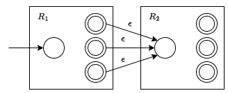
- $R = {R_1}^\star$ - Adds an initial accepting state because $R^\star$ accepts $\epsilon$ and adds epsilon transitions from the finishing states to the start state to represent multiple matches.
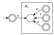
This method of converting regular expressions to NFAs is called Thompson's construction algorithm.
It is also possible to convert an NFA to a regular expression by eliminating state and replacing transitions with regular expressions.
Generalised NFAs
A GNFA is an NFA with regular expressions as transitions.
More formally, a generalised non-deterministic finite automaton (GNFA) is a 5-tuple $(Q, \Sigma, \delta, q_0, q_f)$ where
- $Q$ is the finite set of states
- $\Sigma$ is the input alphabet
- $\delta: (Q \setminus \{q_f\}) \times (Q \setminus \{q_0\}) \rightarrow R$ where $R$ is the set of all regular expressions over the alphabet
- $q_0$ is the start state
- $q_f$ is the accept state
For every $q \in Q \setminus \{q_0, q_f\}$:
- $q$ has outgoing arcs to all other states except $q_0$
- $q$ has incoming arcs from all other states except $q_f$
- $q$ has a self-loop
The run of a GNFA on a word $s \in \Sigma^\star$ is a sequence of states $r_0, r_1, ..., r_n$ such that $r_0 = q_0$ and $\exists s_1,s_2,...s_n \in \Sigma^\star$ such that $s = s_1s_2...s_n$ and $\forall i \in [n]$, $s_i \in L(\delta(r_{i-1}, r_i))$. The definition of accepting run and language are the same as usual.
Every NFA can be converted to an equivalent GNFA.
- Make a new unique start and final state for the NFA using $\epsilon$ transitions
- Add all possible missing transitions out of $q_0$ and into $q_f$ and into/out of all other states including self loops, all labelled $\emptyset$.
Non-regular languages
Non-regular languages can not be expressed using a finite number of states. Consider the extended transition function, $\hat{\delta}$. Starting at $q_0$, it is possible for multiple words to finish at the same end state, or alternatively $\hat{\delta}(q_0, s_1) = \hat{\delta}(q_0, s_2)$ for two strings $s_1$ and $s_2$. Words in a language can then be grouped based on their ending state and there will be a finite number of these groups (this is an equivalence relation and the groups are equivalence classes).
Strings $x$ and $y$ are distinguishable by a language $L$ if there is a string $z$ such that $xz \in L$ but $yz \notin L$ or vice versa. The string $z$ is said to distinguish $x$ and $y$.
If strings $x$ and $y$ are indistinguishable this can be denoted $x \equiv_L y$. $\equiv_L$ is an equivalence relation. The index of $\equiv_L$ is the number of equivalence classes of the relation.
If $L$ is a regular language then $\equiv_L$ has a finite index. Therefore is $\equiv_L$ has infinite index, $L$ must be non-regular.
Myhill-Nerode Theorem
$L$ is a regular language if and only if $\equiv_L$ has a finite index.
To prove a language $L$ is non-regular
- provide an infinite set of strings
- prove that they are pairwise distinguishable by L
This will prove that all strings lie in distinct equivalence classes of $\equiv_L$ and so $\equiv_L$ must have an infinite number of equivalence classes.
Example proof
The language $\{a^n,b^n,c^n\;|\;n\geq 0\}$ over $\{a, b,c\}$ is not regular.
- Consider the infinite set of strings generated by $a^\star$.
- For any $a^i$, $a^j$ where $i \neq j$, observe that $a^i \cdot a^{m-i}b^mc^m = a^mb^mc^m$, which is in $L$, while $a^j \cdot a^{m-i}b^mc^m \notin L$.
- This implies that the set of strings generated by $a^\star$ is pairwise distinguishable by $L$, and so $L$ has infinite index, implying that $L$ must be non-regular by the Myhill-Nerode theorem.
Pumping lemma
If there is a cycle that is reachable from the start state and which can reach an accept state in the state diagram of the DFA $M$ then $L(M)$ is infinite.
The Pumping Lemma
If $L$ is a regular language, then $\exists m>0$ such that $\forall w \in L$ such that $|w| \geq m$, there exists a decomposition $w = xyz$ such that $|y| > 0$, $|xy|\leq m$ such that $\forall i \geq 0$, $xy^iz \in L$.
A language $L$ is an irregular if $\forall m > 0$ such that $\exists w \in L$ such that $|w| \geq m$, such that for all decompositions of $w$ such that $|y| > 0$, $|xy|\leq m$ such that $\forall i \geq 0$, $xy^iz \in L$.
Proof using the pumping lemma follows 4 steps
- Suppose $L$ is regular and let $m$ be the pumping length of $L$
- Choose a string $w \in L$ such that $|w| \geq m$
- Let $w = xyz$ be an arbitrary decomposition of $w$ such that $|xy| \leq m$ and $|y| > 0$
- Carefully pick and integer $i$ and argue that $xyz \notin L$
Example proof
The language $\{a^nb^nc^n\;|\;n\geq 0\}$ over $\{a,b,c\}$ is not regular.
Let $L$ denote this language and for a contradiction, suppose that $L$ is regular and let $m$ be its pumping length. Let $w=a^mb^mc^m \in L$ and let $w = xyz$ where $|xy| \leq m$ and $|y| > 0$. Then $x = a^\alpha$, $y = a^\beta$ and $z = a^\gamma b^mc^m$ for some $\alpha$, $\beta$, $\gamma$ where $\alpha+\beta+\gamma = m$ and $\beta > 0$. Observe that $xy^0z = a^{\alpha + \gamma}b^mc^m$ where $\alpha + \gamma < m$ implying that $xy^0z \notin L$, a contradiction to the pumping lemma. This proves that $L$ is not regular.
Any regular language will satisfy the pumping lemma. A language which satisfies the pumping lemma is not necessarily regular. The pumping lemma can't be used to prove regularity but a regular language will satisfy the pumping lemma.
The pumping length of a regular language is the number of states in its equivalent DFA.
Grammars
A grammar can be denoted as $G = (V, \Sigma, R, S)$ where
- $V$ is a finite set of variables or non-terminals
- $\Sigma$ is a finite alphabet
- $R$ is a finite set of production rules or productions
- $S \in V$ is the start variable
Production rules are of the form $\alpha \rightarrow \beta$ where $\alpha, \beta \in (V \cup \Sigma)^\star$.
An example of a grammar is $G = (\{S\}, \{0,1\}, R, S)$ where $R$ is
- $S \rightarrow 0S1$
- $S \rightarrow \epsilon$
The string 000111 can be derived from the grammar $G$. $S \Rightarrow 0S1 \Rightarrow 00S11 \Rightarrow 000S111 \Rightarrow 000111$. This can be denoted more concisely as $S \overset{*}{\Rightarrow} 000111$.
For each step the string on the left yields the string on the right, so $0S1$ yields $00S11$.
More generally, for every $\alpha, \beta \in (V \cup \Sigma)^\star$ where $\alpha$ is non-empty
- $\alpha \Rightarrow \beta$ if $\alpha$ can be rewritten as $\beta$ by applying a production rule.
- $\alpha \overset{*}{\Rightarrow} \beta$ if $\alpha$ can be rewritten as $\beta$ by applying a finite number of production rules in succession.
The language of a grammar is defined as $L(G) = \{w \in \Sigma^\star \;|\; S \overset{*}{\Rightarrow} w\}$. This is the set of all strings in $\Sigma^\star$ that can be derived from $S$ using finitely many applications of the production rules in $G$.
The language of the example grammar above is $L(G) = \{0^n1^n \;|\;n \geq 0\}$.
The language of the grammar with $R: S \rightarrow S$ is the empty set, as there are no strings in $\Sigma^\star$ which can be derived from it.
A leftmost derivation is one in which successive derivations are first applied to the leftmost variable. A rightmost derivation is the opposite.
A parse tree can be used to represent a derivation. The start variable is the root node, then each variable derived from a production rule are the children.
A grammar is ambiguous if it can generate the same string with multiple parse trees. Equivalently, a grammar is ambiguous if the same string can be derived with two leftmost derivations.
Some ambiguous grammars can be rewritten as an equivalent unambiguous grammar. Those that can't are called inherently ambiguous. It is not possible to decide if a grammar is ambiguous.
Chomsky hierarchy of grammars
For some grammar $G$ where
- $V = \{A,B\}$
- $\alpha, \beta, \gamma, w \in (V \cup \Sigma)^\star$
- $x \in \Sigma^\star$
the hierarchy is
- Type 3: Regular right/left linear - Either $A \rightarrow xB$ and $A \rightarrow x$ (right) or $A \rightarrow Bx$ and $A \rightarrow x$ (left).
- Type 2: Context free - $A \rightarrow w$
- Type 1: Context sensitive - $\alpha A\gamma \rightarrow \alpha \beta \gamma$
- Type 0: Recursively enumerable - $\alpha \rightarrow \beta$
For a strictly regular language, $x \in \Sigma \cup \{\epsilon\}$.
Converting a DFA to a grammar
To convert a DFA to a grammar, let the variables be the states and the start variable be the start state. The rules are then the strings that will go to some accept state starting from each state.
More formally, given a DFA $M = (Q, \Sigma, q_0, F, \delta)$, the equivalent (strictly right-linear) grammar $G = (V, \Sigma, R, S)$ is given by $V = Q$, $S = q_0$ and $R:$
- $\forall q, q' \in Q, a \in \Sigma$ if $\delta(q,a) = q'$ then add rule $q \rightarrow aq'$
- $\forall q \in F$ add rule $q \rightarrow \epsilon$
If $\forall s \in \Sigma^\star$, $q \in Q$ then $\hat{\delta}(q,s) \in F$ if and only if $q \overset{\star}{\Rightarrow} s$. $s \in L(M)$ iff $\hat{\delta}(q_0, s) \in F$ iff $q_0 \overset{\star}{\Rightarrow} s$ iff $s \in L(G)$.
To generate a left-linear grammar, consider all strings from the start state to each state.
The same processes work for converting NFAs to right/left-linear grammars.
Pushdown automata
Context-free languages can't be generated by any of the methods seen so far. A pushdown automaton is a finite automaton with a stack which can generate context-free languages.
Formally, a pushdown automaton (PDA) is a 6-tuple $(Q, \Sigma, \Gamma, \delta, q_0, F)$ where $\Gamma$ is a finite state of the stack alphabet. It includes $\Sigma$ and usually the empty stack symbol, which is $. $\delta$ is defined as $\delta: Q \times \Sigma_\epsilon \times \Gamma_\epsilon \rightarrow 2^{Q \times \Gamma_\epsilon}$. By default, a PDA is non-deterministic.
Transitions in PDAs are denoted $a, c \rightarrow b$ which means read $a$, pop $c$ and push $b$ to move from one state to the next. Something is always read, popped and pushed, but it may be the empty string meaning no change. $b$ can be a string and the leftmost symbol will be on top of the stack.
Formally, the strings accepted by a PDA $(Q, \Sigma, \Gamma, \delta, q_0, F)$, $w \in \Sigma^\star$, must satisfy
- $\exists w_1, ...,w_r \in \Sigma \cup \{\epsilon\}$
- $\exists x_0, x_1, ... x_r \in Q$
- $\exists s_0, s_1, ..., s_r \in \Gamma^\star$
such that
- $w = w_1w_2...w_r$
- $x_0 = q_0$, $s_0 = \epsilon$
- $x_r \in F$
- $\forall i \in [r-1]$, $\delta(x_i, w_{i+1}, a) \ni (x_{i+1}, b)$ where $s_i = at$, $s_{i+1} = bt$ for some $a, b \in \Gamma \cup \{\epsilon\}$ and $t \in \Gamma^\star$.
The run of a PDA on a word $w = a_1...a_r$ is defined as a sequence $(q_0,s_0),...,(q_r,s_r)$ where
- each $q_i$ is a state of $M$
- each $s_i$ is a string over $\Gamma$
- $q_0$ is the start state of the automaton and $s_0$ is the empty string
- for every $i \in [r-1]$, there is a valid transition from $q_i$ with stack contents $s_i$ to $q_{i+1}$ with stack contents $s_{i+1}$ upon reading the symbol $a_{i+1}$.
A run is accepting if the last state in the sequence is accepting.
Pushdown automata accept precisely the set of context-free language. It can be proven that any pushdown automata can be converted to a context-free language and any context-free language can be converted to a pushdown automata.
Context-free grammar to PDA
The construction of a PDA from a CFG uses 3 states
- start state $q_s$
- loop state $q_l$ (simulates grammar rules)
- accept state $q_a$
Example
$G = (\{S\}, \{0,1\}, R, S)$ with $R:$
- $S \rightarrow 0S1$
- $S \rightarrow \epsilon$
The transition from $q_s$ to $q_l$ will be $\epsilon, \epsilon \rightarrow S$$.
The loop transitions will be
- $\epsilon, S \rightarrow 0S1$
- $\epsilon, S \rightarrow \epsilon$
- $0, 0 \rightarrow \epsilon$
- $1, 1 \rightarrow \epsilon$
The transition from $q_l$ to $q_a$ will be $\epsilon, $ \rightarrow \epsilon$.
PDA to CFG
A PDA needs to be normalised before it can be converted to a CFG. A normalised PDA
- has a single accept state
- empties its stack before accepting
- only has transitions that either push a symbol onto the stack (a push move) or pop one off the stack (a pop move) but does not do both at the same time.
To convert a normalised PDA to a CFG, create a variable $A_{pq}$ for each pair of states $p$ and $q$. $A_{pq}$ generates all strings that go from state $p$ with an empty stack to state $q$ with an empty stack.
The rules to generate CFG from a PDA are
- For each $p \in Q$ put the rule $A_{pp} \rightarrow \epsilon$ in $G$
- For each $p,q,r \in Q$ put the rule $A_{pq} \rightarrow A_{pr}A_{rq}$ in $G$
- For each $p,q,r,s \in Q$, $u \in \Gamma$ and $a,b \in \Sigma_\epsilon$ if $\delta(p,a,\epsilon)$ contains $(r,u)$ and $\delta(s,b,u)$ contains $(q, \epsilon)$ put the rule $A_{pq} \rightarrow aA_{rs}b$ in $G$.
CYK bottom up parsing for CFGs in Chomsky Normal Form
A grammar $G = (V, \Sigma, R, S)$ is in Chomsky Normal Form if every production has one of the following shapes:
- $S \rightarrow \epsilon$
- $A \rightarrow x$ ($x \in \Sigma$ is a terminal)
- $A \rightarrow BC$ ($B, C \in V$ where $B, C \neq S$)
The Cocke-Younger-Kasami (CYK) algorithm is a dynamic programming algorithm which builds a table of variables and substrings to work out if a string is generated by a CFG.
Consider a CFG $G = (V, \Sigma, R, S)$. Let $LHS(a) = \{J \in V \;|\; G \text{ has a rule } J \rightarrow a\}$. Let $w = y_1, y_2,...y_l$ and $w[1] = y_1, w[2] = y_2, w[l] = y_l$.
The algorithm is initialised with $M[1, i] = LHS(w[i]) \quad \forall i \in [l]$.
Let $LHS(P \times Q) = \{J \in V \;|\; G \text{ has a rule } J \rightarrow XY \text{ where } X \in P \text{ and } Y \in Q\}$.
The algorithm is then
for i = 2 to l
    for j = 1 to l-(i-1)
        for p = 1 to i-1
            M[i,j] = M[i,j] ∪ LHS(M[p,j] × M[i-p, j+p])
$w$ can be derived from $G$ if and only if $M[l, 1]$ contains the start state $S$.
The time complexity of the algorithm is $O(n^3)$ where $n$ is the length of the string.
Converting to Chomsky normal form
Any context-free language is generated by a context-free grammar in Chomsky normal form.
A grammar $G = (V, \Sigma, R, S)$ can be converted to Chomsky normal form by doing the following
- Create a new start variable $S_0$ and add $S_0 \rightarrow S$
- Eliminate $A \rightarrow \epsilon$ productions where $A \neq S$
- Eliminate unit productions $A \rightarrow B$
- Add new variables and productions to eliminate remaining violations of the rules with more than two variables or two terminals.
Example
- $S \rightarrow ASB$
- $A \rightarrow aAS | a | \epsilon$
- $B \rightarrow SbS | A | bb$
- Add rule $S_0 \rightarrow S$
- For each rule with $A$, add a new rule with $A = \epsilon$ to eliminate $A \rightarrow \epsilon$. The rules are now
- $S_0 \rightarrow S$
- $S \rightarrow ASB | SB$
- $A \rightarrow aAS | a | aS$
- $B \rightarrow SbS | A | bb | \epsilon$
- This introduces $B \rightarrow \epsilon$ which can be removed the same way, giving
- $S_0 \rightarrow S$
- $S \rightarrow ASB | SB | AS | S$
- $A \rightarrow aAS | a | aS$
- $B \rightarrow SbS | A | bb$
- Eliminate unit productions. Firstly, replace $A$ with its RHS in the rule for $B$
- $S_0 \rightarrow S$
- $S \rightarrow ASB | SB | AS | S$
- $A \rightarrow aAS | a | aS$
- $B \rightarrow SbS | aAS | a | aS | bb$
- Eliminate $S \rightarrow S$ and replace the RHS of $S_0$ with $S$
- $S_0 \rightarrow ASB | SB | AS$
- $S \rightarrow ASB | SB | AS$
- $A \rightarrow aAS | a | aS$
- $B \rightarrow SbS | aAS | a | aS | bb$
- Eliminate RHS with more than 2 variables by creating new rules
- $S_0 \rightarrow AU_1 | SB | AS$
- $S \rightarrow AU_1 | SB | AS$
- $A \rightarrow aU_2 | a | aS$
- $B \rightarrow SU_3 | aU_2 | a | aS | bb$
- $U_1 \rightarrow SB$
- $U_2 \rightarrow AS$
- $U_3 \rightarrow bS$
- Replace terminal-variable rules with extra rules
- $S_0 \rightarrow AU_1 | SB | AS$
- $S \rightarrow AU_1 | SB | AS$
- $A \rightarrow V_1U_2 | a | V_1S$
- $B \rightarrow SU_3 | V_1U_2 | a | V_1S | V_2V_2$
- $U_1 \rightarrow SB$
- $U_2 \rightarrow AS$
- $U_3 \rightarrow V_2S$
- $V_1 \rightarrow a$
- $V_2 \rightarrow b$
- This grammar is now in Chomsky normal form
Advantages of having a CFG in Chomsky normal form:
- the CYK algorithm can be used to parse strings in polynomial time
- every string of length $n$ can be derived in exactly $2n-1$ steps
Testing is a CFG produces and empty language
To test if the language generated by a CFG is empty
- Find and mark all variables with a terminal or $\epsilon$ on the right hand side
- Mark any variable $A$ for which there is a production $A \rightarrow w$ where $w$ comprises of only marked variables and terminals.
- Repeat 2. until no new variables get marked.
- If $S$ is unmarked, the language is empty.
Proving a language is context-free
The pumping lemma can be used to prove a language is regular. A variation of the pumping lemma can be used to prove a language is context-free. If $L$ is a context-free language, then $\exists m > 0$ such that $\forall w \in L: |w| \geq m, \exists$ a decomposition $w=uvxyz$ such that $|vy|>0$, $|vxy| \leq m$, $\forall i \geq 0$, $uv^ixy^iz \in L$.
The pumping length for a CFL is $m = b^{|V| + 1}$ where $b$ is the longest right hand side of a rule in the grammar and $|V|$ is the number of variables.
To prove a language is not context-free, assume it is context-free and show a contradiction.
Example
$L = \{a^nb^nc^n \;|\; n>0\}$ is not a CFL.
Assume that $L$ is a CFL and $m$ be its pumping length. Since $|vxy|\leq m$ and $|vy|>0$ it follows that $|vxy|$ contains at least one symbol from $\{a, b, c\}$ and at most 2. So $uv^0xy^0z \notin L$ as the number of each type of symbol can't be equal. This contradicts the pumping lemma so $L$ is not a CFL.
Testing is a CFG is finite
If a grammar contains no strings of length longer than the pumping length $m$ the language is finite.
If a grammar contains a string of length longer than $m$ it contains a string of length at most $2m-1$.
To check if a CFG is finite, generate all strings of length $m < l < 2m$ and use the CYK algorithm to check if they can be generated by the grammar. If any string can is generated by the grammar then its language is infinite.
Closure properties for CFLs
Context-free languages are closed under
- union
- concatenation
- Kleene closure
Context-free languages are not closed under
- intersection
- complementation
The intersection of a CFL with a regular language is a CFL. Let $M_1 = (Q_1, \Sigma, q_1, F_1, \delta_1)$ and $M_2 = (Q_2, \Sigma, \Gamma, q_2, F_2, \delta_2)$. Define their intersection be denoted $M = (Q, \Sigma, \Gamma, q, F, S)$ where
- $Q = Q_1 \times Q_2$
- $q = (q_1, q_2)$
- $F = F_1 \times F_2$
- $\forall a \in \Sigma, b \in \Gamma, \alpha \in Q_1, \beta \in Q_2$ we have $\delta((\alpha, \beta), a, b) \ni ((\alpha', \beta'), c)$ where $(\beta', c) \in \delta_2(\beta, a, b)$ and $\alpha' = \alpha$ if $a = \epsilon$ and $\delta_1(\alpha, a)$ otherwise.
Turing machines
A Turing machine consists of an infinite memory tape and a reading head which points to an item in memory. The reading head can either be moved left or right.
Formally, a Turing machine is a 7-tuple $(Q, \Sigma, \Gamma, \delta, q_0, q_\text{accept}, q_\text{reject})$ where $Q, \Sigma, \Gamma$ are all finite sets and
- $Q$ is the set of states
- $\Sigma$ is the input alphabet not containing the blank symbol $\sqcup$
- $\Gamma$ is the tape alphabet $\sqcup \in \Gamma$ and $\Sigma \subseteq \Gamma$
- $\delta: Q \times \Gamma \rightarrow Q \times \Gamma \times \{L, R\}$ is the transition function
- $q_0 \in Q$ is the start state
- $q_\text{accept} \in Q$ is the accept state
- $q_\text{reject} \in Q$ is the reject state where $q_\text{reject} \neq q_\text{accept}$
The $\vdash$ symbol denotes the start of the tape.
Transitions in a Turing machine are denoted $a \rightarrow b, L$ which means if the symbol pointed to by the reading head is $a$ then replace it with $b$ and move the reading head left. The third symbol can also be $S$ for stay on the current symbol, which could be expressed using multiple $L/R$ transitions but is used for convenience.
Turing machine terminology
- The configuration of a Turing machine is a snapshot of what the machine looks like at any point. $X = (u,q,v)$ is a configuration where $q$ is the current state, $u$ is the contents of the tape up to $q$ and $v$ is the contents of the tape after and including $q$.
- Configuration $X$ yields configuration $Y$ if the Turing machine can legally go from $X$ to $Y$ in one step.
- The start configuration is $(\vdash, q_0, w)$
- The accepting configuration is $(u, q_\text{accept}, v)$
- The rejecting configuration is $(u, q_\text{reject}, v)$
- Accepting or rejecting configurations are called halting configurations
- The run of a Turing machine $M$ of a string $w$ is a sequence of configurations $C_1, ..., C_r$ such that $C_1$ is the start configuration and for $i$ from $1$ to $r-1$ configuration $C_i$ yields $C_{i+1}$
- An accepting run is a run in which the last configuration is an accepting configuration
- A Turing machine can either halt and reject, halt and accept or not halt for an input
- The language accepted by a Turing machine is the set of words that are accepted by the machine
- A language is Turing-recognisable if it is the language accepted by some Turing machine. These are also called recursively enumerable and are generated by Chomsky type-0 grammars.
- A Turing machine that halts is called a decider ot total Turing machine. For a decider/total Turing machine $M$, $L(M)$ is the language decided by $M$.
- A language is Turing decidable if it is the language accepted by some decider/total Turing machine.
Adding multiple tapes, multiple heads or using bidirectional infinite tapes does not increase the power of the Turing machine model. All of these features can be expressed using a single tape with a single head.
Enumeration machines or enumerators are Turing machines with a dedicated output tape. It consists of a finite set of states with a special enumeration tape, a read/write work tape and a write-only output tape. It always starts with a blank work tape.
When it enters an enumeration state, the word in the output tape is enumerated. The machine erases the output tape, sends the write-only head back to the start, leaves the work tape untouched and continues. The language of an enumerator is the set of words enumerated by the machine. A language is Turing recognisable if and only if it is enumerated by some enumerator. Therefore recursively enumerable is the same as Turing recognisable.
To convert a Turing machine $M$ to an enumerator, for each $i = 1, 2, 3, ...$, run $M$ for $i$ steps on each input $s_1, s_2, ..., s_i$ and if any computations accept, print out the corresponding $s_j$.
A universal turing machine $U$ takes as input the string "Enc(M)#w" and simulates machine $M$ on word $w$. The input string is also denoted $\left<M, w\right>$.
Halting and membership problems
The halting problem is defined as $HP = \{\left<M,x\right>\;|\;M \text{ halts on } x\}$.
The halting problem is Turing-recognisable as the universal Turing machine can be used to run $\left<M, x\right>$. The halting problem is not decidable and this can be proven by contradiction.
Consider an infinite matrix where each row is a binary-encoded Turing machine and the columns are input strings. Each cell contains either $L$ or $H$ if the machine either loops or halts on the input. This matrix should contain every Turing machine.
Suppose there is a decider $N$ for the halting problem, then we can construct a Turing machine which is not present in the matrix, a contradiction. On input $\left<M, x\right>$ the machine $N$ halts and accepts if it determines that $M$ halts on input $x$ or halts and rejects if it determines that $M$ does not halt on input $x$.
Consider a Turing machine $K$ which on input $y$ writes $\left<M_y, y\right>$ (this corresponds to the diagonal of the matrix) on the input tape and simulates the run of the string $\left<M_y, y\right>$ on $N$ and finally halts and accepts if $N$ rejects or goes into an infinite loop if $N$ accepts.
The output of $K$ is the opposite of $N$ on the original matrix. Therefore $K$ cannot exist in the original matrix, but this matrix contains every turing machine, a contradiction. Therefore the halting problem is undecidable.
The membership problem is defined as $MP = \{\left<M,x\right>\;|\;x \in L(M)\}$. The membership problem is Turing-recognisable as the universal Turing machine can be used to simulate it.
The membership problem is undecidable. Suppose the membership problem is decidable and let $N$ be a decider for it. It can be shown that $N$ can be used to construct a decider $K$ for the halting problem, which is a contradiction as we have shown the halting problem is undecidable.
Consider a Turing machine $K$ that on input $\left<M, x\right>$ constructs a new machine $M'$ obtained from $M$ by adding a new accept state to $M$ and making all incoming transitions to the old accept and reject states go to the new accept state. The machine then simulates $N$ on input $\left<M', x\right>$ and accepts if $N$ accepts. As $N$ is undecidable, the membership problem is also undecidable. This is a reduction from the halting problem to the membership problem to show undecidability.
Reductions
For $A \subseteq \Sigma^$, $B \subseteq \Delta^$, $\sigma: \Sigma^* \rightarrow \Delta^$ is called a (mapping) reduction from $A$ to $B$ if for all $x \in \Sigma^, x \in A \iff \sigma(x) \in B$ and $\sigma$ is a computable function.
$\sigma$ is a computable function if there is a decider that, on input $x$, halts with $\sigma(x)$ written on the tape.
Consider an instance of the halting problem $\left<M, x\right>$. Define a Turing machine $M_x'(y)$ such that $y$ is ignored and $M$ is simulated on input $x$. If $M$ halts then accept. This is a mapping reduction from the halting problem to the membership problem.
$\left<M, x\right> \in HP \iff \left<M'_x,x\right> \in MP$. This means that if there is a decider for the membership problem, there is a decider for the halting problem as well.
Using reductions, other problems can be proved undecidable
- $\epsilon$-acceptance = $\{\left<M\right> \;|\; \epsilon \in L(M)\}$
- $\exists$-acceptance = $\{\left<M\right> \;|\; L(M) \neq \emptyset\}$
- $\forall$-acceptance = $\{\left<M\right> \;|\; L(M) = \Sigma^*\}$
The same reduction as for the membership problem can be used for these three problems.
Therefore $\left<M, x\right> \in HP$ if and only if
- $\left<M'_x,x\right> \in MP$
- $\left<M'_x\right> \in \epsilon$-acceptance
- $\left<M'_x\right> \in \exists$-acceptance
- $\left<M'_x\right> \in \forall$-acceptance
As there does not exist a decider for the halting problem, none of these problems are decidable.
If $A \leq_mB$ and
- $B$ is decidable then $A$ is decidable
- $A$ is undecidable then $B$ is undecidable
- $B$ is Turing-recognisable then $A$ is Turing-recognisable
- $A$ is not Turing-recognisable then $B$ is not Turing-recognisable
A language is decidable if and only if $L$ and $\overline{L}$ are both Turing-recognisable.
Proof forwards: If $L$ is decidable, then $L$ is Turing-recognisable by definition. $\overline{L}$ is everything that is not accepted by the decider for $L$, so is itself decidable and therefore Turing-recognisable.
Proof backwards: If $L$ and $\overline{L}$ are both Turing-recognisable with recognisers $P$ and $Q$ then a decider $M$ will run both $P$ and $Q$ on the input $x$. If $P$ accepts then halt and accept, if $Q$ accepts then halt and reject. $M$ is a decider for $L$.
The complement of the halting problem is not Turing-recognisable because if it was, then the halting problem and its complement would be recognisable which by the theorem above would make the halting problem decidable, which it is not.
Closure properties of Turing-recognisable and decidable languages
Both Turing-recognisable and decidable languages are closed under
- union
- intersection
- Kleene closure
- concatenation
Decidable languages are closed under complementation but Turing-recognisable languages are not as seen with the complement of the halting problem.
Languages classes
Regular languages are a subset of context-free languages are a subset of decidable languages. Decidable languages are the intersection of Turing-recognisable and co-Turing-recognisable languages.
Coursework notes (not examinable)
The first two stages of compilation are lexical analysis and syntax analysis.
Lexical analysis breaks source code up into tokens, classifies them, reports lexical errors, builds the symbol table and passes tokens to the parser. The parser does syntax analysis. It uses the grammar of the language to build a parse tree and then an abstract syntax tree.
Some common types of token include keywords, whitespace, identifiers, constants, operators and delimiters.
JavaCC generates a left-to-right top-down parser.
CS260 - Algorithms
Greedy algorithms
Greedy algorithms are those that make locally optimal choices. This means at each step the algorithm selects the best option available at the time, not considering the effect this will have on future choices.
Greedy algorithms covered:
- Interval scheduling
- Interval partitioning
- Scheduling to minimise maximum lateness
- Dijkstra's shortest path algorithm
- Minimum spanning tree algorithms
Interval Scheduling
Input A set of intervals, ${1,2,...,n}$ with start time $s(i)$ and finish time $f(i)$.
Output The largest subset of compatible intervals. Compatible intervals are those that do not overlap in time, that is $f(i) \leq s(j)$ or $f(j) \leq s(i)$.
The algorithm will select an interval using a greedy rule, add it to the schedule and remove all other incompatible intervals.
As pseudocode this would be
I = set of intervals
A = {}
while I is not empty
    select some i from I using the greedy rule
    add i to A
    delete all intervals from I which are incompatible with i
return A
Possible greedy rules for interval scheduling
-
Earliest start time first - This is not optimal if the earliest interval has a long duration. In the example below, the longest interval is selected first, meaning only 1 interval can be scheduled whereas the optimal number is 4.
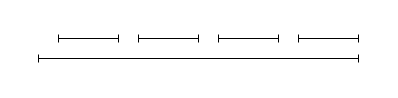
-
Shortest duration first - This is not optimal when the selected interval is incompatible with several longer, compatible intervals, as in the example below.
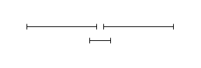
-
Fewest incompatibilities first - This seems like it might work but is not optimal for the example shown below.
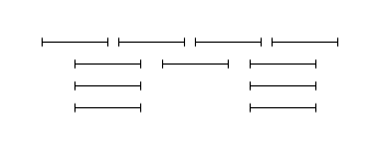
In this example, the middle interval would be selected first, eliminating the two above it. Then one from the left and one from the right would be selected, giving a schedule with 3 intervals. The optimal schedule would consist of the top row of intervals shown above and would have size 4.
-
Earliest finish time first - This rule is optimal.
Proof of optimality
Let $O$ be the optimal set of intervals and $A$ be the earliest finish time first output set. It is not possible to show $O = A$ as there may be several optimal sets for some inputs. Instead, it is shown that $A$ is optimal if $|A| = |O|$.
To prove this, it has to be shown that $A$ "stays ahead" of $O$. This means that some part of $A$ is always at least as good as some part of $O$.
Let $i_1,...,i_k$ be the intervals in $A$ in the order they were added to $A$. Let $j_1, ..., j_m$ be the intervals in the optimal solution $O$. $A$ is optimal if $k = m$. Assume the intervals in $O$ are ordered.
The greedy rule guarantees that $f(i_1) \leq f(j_1)$. It needs to be shown that for each $r \geq 1$ the $r^{th}$ interval in $A$ finishes no later than the $r^{th}$ interval in $O$.
Consider "For all indices $r \leq k$ we have $f(i_r) \leq f(j_r)$". This can be proven by induction. For $r=1$ the statement is true, as the algorithm starts by selecting $i_1$ with the earliest finish time. Assume $f(i_{r-1}) \leq f(j_{r-1})$. Since $O$ consists of compatible intervals, $f(j_{r-1}) \leq s(j_r)$. Combining this with the inductive hypothesis gives $f(i_{r-1}) \leq s(j_r)$. This means the interval $j_r$ was available when the greedy algorithm chose $i_r$, so $f(i_r) \leq f(j_r)$. $\blacksquare$
This shows that the greedy algorithm stays ahead, it can then be shown $k = m$ by contradiction. If $A$ is not optimal, an optimal set must have more intervals scheduled, that is $m > k$. Using the result of the last proof with $r = k$, $f(i_k) \leq f(j_k)$. Since $m > k$, there is a request $j_{k+1}$ in $O$. This request must end after $j_k$ ends and hence after $i_k$ ends. This means after deleting the set of intervals incompatible with $i_1,...,i_k$, the set of possible intervals $I$ still contains $j_{k+1}$. The greedy algorithm stops with request $i_k$ but it can only stop when $I$ is empty, a contradiction. $\blacksquare$
Complexity
Interval scheduling can be implemented more efficiently using the following algorithm:
sort I in order of finishing time
A = {I[1]}
for j in I
    if s(j) > f(A[-1]) then
        A += j
This has time complexity $O(n\log n)$ for sorting and $O(n)$ for iteration, giving overall $O(n\log n)$.
Interval Partitioning
Input A set of intervals, ${1,2,...,n}$ with start time $s(i)$ and finish time $f(i)$.
Output All intervals scheduled using the fewest possible resources.
The number of resources needed is at least the depth of the set of intervals. The depth is given by the maximum number of intervals which pass over a single point in time. Therefore the optimal solution will at least as many resources as the depth.
The algorithm for interval partitioning is as follows:
sort intervals by start time
for each interval
    if interval is compatible with an existing resource
        add it to the existing resource
    else
        create a new resource
        add it to the new resource
Scheduling to Minimise Lateness
Input $n$ jobs consisting of pairs of (duration, deadline).
Output Schedule of jobs that minimises maximum lateness.
The algorithm needs to determine the start time of and interval, $s(i)$. The finish time, $f(i)$ is then given by $s(i) + t_i$ where $t$ is the duration. The lateness of a request is given by $l_i = f(i) - d_i$ where $d$ is the deadline. The goal of the algorithm is to schedule the jobs in order to minimise the maximum lateness of all jobs, $L$.
Greedy rules for minimising maximum lateness
- Schedule the jobs in order of increasing length $t_i$ to get the short jobs done quickly. This is not optimal, as a job with a shorter time and very long deadline will be scheduled before a job with duration = deadline.
- Let the slack time of a job be given by $d_i - t_i$. Scheduling the jobs by smallest slack time does not work. Consider jobs $t_1 = 1$, $d_1 = 2$ and $t_2 = 10$, $d_2 = 10$. Using minimum slack, job 2 will be scheduled first, giving total lateness 9, whereas scheduling job 1 first will give total lateness 1.
- Earliest deadline first - This is the optimal rule.
The pseudocode for this algorithm is as follows:
sort jobs by earliest deadline first
let f = s
for each job i
    assign job i to time interval s(i) = f to f(i) = f + t_i
    let f = f + t_i
return the set of scheduled intervals [s(i), f(i)]
Proof of optimality
Consider a schedule $A$ output by the algorithm and an optimal schedule $O$. It is possible to transform $O$ into $A$ without affecting its optimality using an exchange argument.
A schedule is said to have an inversion if a job $i$ with deadline $d_i$ is scheduled before another job $j$ with earlier deadline $d_j < d_i$. By definition $A$ does not contain any inversions. It is then possible to show that all schedules with no inversions and no idle time have the same maximum lateness.
$A$ is optimal if it can be shown an optimal schedule with inversions can be converted into $A$ without increasing the maximum lateness.
If $O$ has an inversion, there is a pair of adjacent, inverted jobs $i$ and $j$. Swapping these jobs decreases the number of inversions by 1. It is then possible to prove the new swapped schedule has a maximum lateness no larger than that of $O$.
For the schedule $O$, let each request $r$ be scheduled for the interval $[s(r), f(r)]$ with lateness $l'_r$. Let $L' = \max_rl'_r$ denote the maximum lateness of $O$.
Let $\bar{O}$ denote the swapped schedule and $\bar{s}_r, \bar{f}_r, \bar{l}_r$ and $\bar{L}_r$ denote the corresponding properties.
The finish time of $j$ before the swap is exactly equal to the finish time of $i$ after the swap. Therefore all other jobs finish at the same time in both schedules. As $j$ finishes earlier in $\bar{O}$ and $d_i > d_j$ the swap can't increase the lateness of $j$.
After the swap, job $i$ finishes at time $f(j)$. If job $i$ is late in $\bar{O}$, then its lateness is $\bar{l}_i = \bar{f}(i) - d_i = f(j) - d_i$. Since $d_i > d_j$, $\bar{l}_i = f(j) - d_i < f(j) - d_j = l'_j$. The lateness in $O$ is $L' \geq l'_j > \bar{l}_i$, so the swap does not increase the maximum lateness of the schedule. Therefore any optimal solution with inversions can be transformed into $A$ without increasing the maximum lateness, so $A$ is optimal. $\blacksquare$
Complexity
Sorting is $O(n\log n)$ and iteration is $O(n)$ giving $O(n\log n)$ overall.
Dijkstra's Algorithm
Input Directed weighted graph with non-negative weights and a source node
Output The shortest path and length from the source node to every other
Dijkstra's algorithm starts at the source node and selects the unexplored node which results in a shortest path at each step.
Dijkstra's algorithm can be represented in pseudocode as follows
s = start node
G = (V, E) = graph
S = {s} = set of explored vertices
d = shortest path distance
d(s) = 0
while S != V
    select v not in S which minimises d'(v)
    add v to S and let d(v) = d'(v)
where $d'(v) = \min_{e = (u,v):u\in S} d(u) + \ell_e$.
To produce the shortest paths the edge chosen at each step should be recorded when $v$ is added to $S$. Then to find the shortest path to some node $x$ look at the edge chosen, $(y,x)$, for example. Then look at the edge chosen for $y$ and recursively follow the path back to the source.
Proof of correctness
Dijkstra's is correct if after each iteration $\forall u \in S$, $P_u$ is a shortest path from $s$ to $u$ and $d(u) = \ell(P_u)$.
This can be proven by induction on the size of $S$.
Base case $|S| = 1$, $S = {s}$ and $d(s) = 0$
Inductive case Suppose the claim holds when $|S| = k$ for some $k \geq 1$.
For $|S| = k+1$, add the node $v$. Let $(u,v)$ be the final edge of the path $P_v$. By the inductive hypothesis, $P_u$ is the shortest path for each $u \in S$.
Consider any other $s$-$v$ path $P$. In order to reach $v$, $P$ must leave $S$ somewhere. Let $y$ be the first node on $P$ that is not in $S$ and $x \in S$ be the node just before $y$.
Let $P'$ be the subpath of $P$ from $s$ to $x$. Since $x \in S$, $P_x$ is the shortest path and has length $d(x)$ by the inductive hypothesis. Therefore $\ell(P') \geq \ell(P_x) = d(x)$.
Therefore $\ell(P) \geq \ell(P') + \ell(x,y) \geq d(x) + \ell(x,y) \geq d'(y)$. Since Dijkstra's selected $v$ for this iteration, $d'(y) \geq d'(v) = \ell(P_v)$. Combining these inequalities gives $\ell(P) \geq \ell(P') + \ell(x,y) \geq \ell(P_v)$, so the alternative path is at least as long as the path determined by Dijkstra's. $\blacksquare$
Complexity
Consider a graph with $n$ nodes and $m$ edges. Using the while loop in the pseudocode above gives $n-1$ iterations. Computing the minimum edge would take $O(m)$ time, giving an overall time complexity of $O(mn)$.
This can be improved by using a priority queue with key $d'(v)$ for each node $v \in V \setminus S$. Then the ExtractMin method can be used each iteration to get the smallest $d'(v)$. If $v$ is added to $S$ and there is some node $w$ and an edge $e = (v, w)$ then the new key for $w$ is $\min(d'(w), d(v) + \ell_e)$. The ChangeKey operation can then be used to change the key if necessary.
Using a heap based priority queue implementation, both ExtractMin and ChangeKey can be done in $O(\log n)$ time. $O(m)$ time will be needed to populate the priority queue and at most $n$ ExtractMin and $m$ ChangeKey operations will be needed. This results in an overall $O(m\log n)$ time complexity.
Minimum Spanning Tree Algorithms
Input A directed graph with non-negative weights
Output A minimum spanning tree - A tree which contains all nodes of the input graph and is of minimum cost
There are several greedy rules to consider, all of which correctly find minimum spanning trees.
- Start with the vertices from the input and add edges in order of increasing cost, not including those which create a cycle. This is Kruskal's algorithm.
- Start with a root node and add the cheapest node to the existing tree each iteration. This is Prim's algorithm.
- Start with the full graph and remove edges in order of decreasing cost if removing the edge will not make the graph disconnected. This is called the Reverse-delete algorithm.
Proof of the cut set property
The cut set property can be used to prove the correctness of Kruskal's and Prim's algorithms.
Assume all edges have distinct costs. Consider two non-empty, sets $S$ and $V \setminus S$. The edges between these sets is called the cut set. Let $e = (v,w)$ be the minimum cost edge in the cut set. The cut set property states that every minimum spanning tree contains edge $e$.
This can be proven by an exchange argument. Let $T$ be a spanning tree that does not contain $e = (v,w)$. $T$ is a spanning tree, so there must still be a path $P$ from $v$ to $w$. Consider a $v' \in S$ and $w' \in V \setminus S$. Let $e' = (v', w')$ be the edge joining them. $e$ is therefore in the cut set and $P$ is a path from $v$ to $w$ containing $e$.
If $e'$ is exchanged for $e$ this gives a new tree $T' = (T \setminus {e'}) \cup {e}$. $T'$ is connected and acyclic because $T$ was connected and acyclic and $e$ connects the two disjoint trees created by removing $e'$.
As both $e$ and $e'$ are in the cut set, but $e$ is the cheapest edge in the cut set, $c_e < c_{e'}$. This means the total cost of $T'$ is less than that of $T$ because $T'$ contains $e$. $\blacksquare$
Proof of optimality for Kruskal's
Consider any edge $e = (v,w)$ added by Kruskal's algorithm and let $S$ be the set of all nodes to which $v$ has a path just before $e$ is added. At this point, $v \in S$ and $w \not\in S$. This means no edge between $S$ and $S \setminus V$ has been encountered yet. Therefore $e$ is the cheapest edge in the cut set and by the cut set property it belongs to every minimum spanning tree. $\blacksquare$
Proof of optimality for Prim's
In each iteration there is a set $S \subseteq V$ on which a partial spanning tree has been constructed and a node $v$ and edge $e$ of minimum cost. $e$ is therefore the cheapest edge in the cut set, so by the cut set property belongs to every minimum spanning tree. $\blacksquare$
Proof of the cycle property
The cycle property can be used to prove the correctness of the reverse-delete algorithm.
Assume all edge costs are distinct. Let $C$ be any cycle in $G$ and let $e = (v,w)$ be the most expensive edge belonging to $C$. $e$ does not belong to any minimum spanning tree of $G$.
This can be proven by an exchange argument. Let $T$ be a spanning tree that contains $e$. Deleting $e$ from $T$ splits the nodes into to disjoint sets, $S$ containing $v$ and $V \setminus S$ containing $w$. As $e$ was in a cycle, a new path $P$ can be found from $v$ to $w$ by following the cycle. Let $e'$ be the edge in the cut set on this alternative path.
Consider $T' = (T - {e}) \cup {e'}$. Using similar reasoning to the cut set property, $T'$ is a spanning tree of $G$. Since $e$ was the most expensive edge in the cycle $C$ and $e'$ also belongs to $C$, $e'$ must be cheaper than $e$ so $T'$ is cheaper than $T$. $\blacksquare$
Proof of optimality for reverse-delete
Consider any edge $e = (v,w)$ removed by the reverse-delete algorithm. When $e$ is removed it is in a cycle $C$ and since it is the first edge considered in order of decreasing cost it must be the most expensive edge on the cycle. Therefore by the cycle property, it does not belong to any MST. The result is connected, as reverse-delete won't remove an edge which will make the graph disconnected. The result is acyclic as if the graph did contain a cycle, the algorithm would've removed the most expensive edge on it so the result must not contain any cycles. Therefore the result is a MST. $\blacksquare$
Eliminating the assumption of distinct edge costs
By adding extremely small, distinct amounts to the cost of every edge the edge costs are all made distinct. The original ordering of distinct nodes will not change as the amounts added are so small but non-distinct nodes are now distinct and will therefore work with the assumptions made.
Prim's implementation
Prim's algorithm can be efficiently implemented using a priority queue of nodes with the attachment cost as keys, which takes $O(m)$ time to populate. ExtractMin is used to get the cheapest node and ChangeKey is used to update attachment costs. There are $n-1$ ExtractMin and $O(m)$ ChangeKey operations. These can be performed in $O(\log n)$ time for a heap based implementation, giving an overall time complexity of $O(m \log n)$.
Kruskal's implementation
Kruskal's algorithm can be implemented efficiently using a union-find data structure. This data structure maintains disjoint sets and provides two operations, union and find. Find(x) returns the name of the set containing x. If two nodes x and y are in the same set then Find(x) = Find(y). Union(x,y) merges two sets into a single set.
A pointer-based implementation of the union-find data structure can be initialised in $O(n)$, perform Union in $O(1)$ and perform Find in $O(\log n)$ time.
Kruskal's algorithm can be implemented using the union-find data structure as follows:
sort edges by ascending cost
for each vertex v:
    make-set(v)
for each edge e = (u, v):
    if find(u) != find(v):
        union(find(u), find(v))
For a graph with $n$ nodes and $m$ edges, sorting takes $O(m\log m)$, which is $O(n\log m)$ given that $m \leq n^2$. The union-find initialisation takes $O(n)$ and there are $m$ iterations with two finds and a union. Using the pointer based implementation, these take $O(\log n)$ and $O(1)$ time respectively, giving $O(m\log n)$ and $O(m)$ for $m$ iterations.
This gives an overall time complexity of $O(m\log n)$. Even if a more efficient union-find implementation is used, the complexity is still limited by the sorting.
Divide and conquer algorithms
Divide and conquer algorithms work by splitting a larger problem into smaller sub-problems which are then solved recursively and combined to give a solution to the original problem.
Divide and conquer algorithms covered:
Merge Sort
Merge sort sorts a list by dividing it into two halves, sorting each half recursively and then merging the results in $O(n)$ time.
The runtime of merge sort can be represented using a recurrence: $$ T(n) = \begin{cases} O(1) & n \leq 2\\ 2T(n/2) + O(n) & \text{otherwise} \end{cases} $$ This is called the merge sort recurrence. If $n$ is a power of 2, it can be shown that $T(n) = O(n\log n)$.
Consider the recurrence tree:
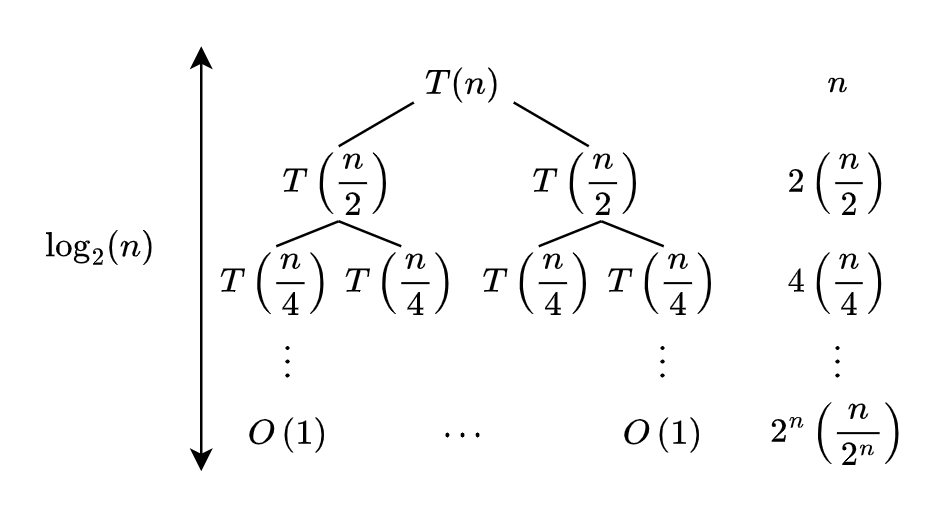
At each level $i$ there are $2^i$ recursive calls taking $T(\frac{n}{2^i})$ time plus the $O(\frac{n}{2^i})$ time to merge for each of the $2^i$ recursive calls, giving $O(n)$ additional work at each level. As the height of the tree is $\log_2(n)$, the overall runtime is $O(n\log_2 n)$ as there is $n$ time taken to merge for $\log_2(n)$ levels. As logarithms of different bases only differ by a constant, the time complexity of merge sort can then be simplified to $O(n \log n)$.
Finding the Closest Pair of Points
Input $n$ points of the form $(x_i, y_i)$
Output The closest pair of points by Euclidean distance
There is a trivial $O(n^2)$ algorithm for this problem which finds the distance between each pair of points.
min = null
for i in points:
    for j in points:
        if i != j and distance(i, j) < distance(min):
            min = (i, j)
There is a more efficient divide and conquer algorithm which can find the closest pair on $O(n\log n)$ time. This solution only considers points with distinct $x$- and $y$-coordinates for simplicity but can be extended to work for any points.
Consider the following:
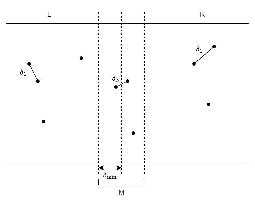
The points are sorted by $x$-coordinate and split into two groups, L and R.
- $\delta_1$ is the distance between the closest pair in L
- $\delta_2$ is the distance between the closest pair in R
- $\delta_3$ is the distance between the closest pair in M
- $\delta_{\min} = \min(\delta_1, \delta_2)$, which in the example above is $\delta_1$.
The closest pair is then given by $\min(\delta_1, \delta_2, \delta_3)$, which in the example above is $\delta_3$.
The region labelled M is the set of points from $L$ and $R$ which are closer to the centre than the closest pair in either half. This region needs to be considered in case the closest pair consists of a point from each side. Anything outside this region will be further apart than the closest pair in both halves so does not need to be considered.
The base case is when the size of a group is 2 or 3. The distances between all of the points can be calculated and the minimum returned.
The algorithm is as follows:
- Sort points by $x$-coordinate
- Split points into two groups of size $n/2$, labelled L and R
- Recursively find the closest pair in each L and R
- Find the closest pair in the region M
- Return the closest of the three pairs from L, R and M.
Steps 1-3 and 5 are straightforward. Step 4 is not.
Consider the region M:
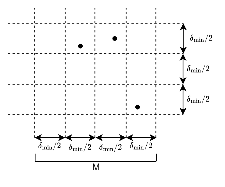
It can be divided into squares of size $\delta_{\min}/2$. There can only be one point in each square as otherwise $\delta_{\min}$ wouldn't be correct.
To find the closest pair, sort the points by $y$-coordinate ascending. The indices of any pair $(i, j)$ in the list where $\delta_{ij} < \delta_{\min}$ will differ by at most 7. I am not entirely sure why, but if they are more than 7 indices apart then their distance is greater than $\delta_{\min}$. For the example above there are only 3 points in M, so the minimum of the distances between them will be returned. If there were 16 points in M each point would only have to be compared to the next 7, not all remaining points.
Using this method, the algorithm is as follows:
- Sort points by $x$-coordinate
- Split points into two groups of size $n/2$, labelled L and R
- Recursively find the closest pair in each L and R. Store the closest pair distance from both halves as $\delta_{\min}$
- Consider points with $x$-coordinates within $\delta_{\min}$ of the centre line, label this set M
- Sort the points in M by $y$-coordinate
- Store an initial value of $\delta_3 = \delta_{\min}$
- Compare distance of each point to the next 7, updating $\delta_3$ is a closer pair is found
- Return the minimum of $\delta_{\min}$ and $\delta_3$
Complexity
The time complexity of finding the closest pair in M $O(n \log n)$ for the sorting and $O(7n) = O(n)$ for the distance comparisons. Given this, the recurrence is $$ T(n) \leq \begin{cases} O(1) & n \leq 3\\ 2T(\frac{n}{2})+O(n\log n) & \text{otherwise} \end{cases} $$ This means $n\log\left(\frac{n}{2^i}\right) = n\log(n) - n\log(2^i)=O(n\log n)$ is done at each level $i$ for a total of $\log_2(n)$ levels, giving an overall time complexity of $O(n\log^2(n))$.
It is possible to merge in $O(n)$ time by presorting the list by $y$-coordinate instead of sorting by $y$-coordinate for each iteration. Changing this in the recurrence above gives the merge sort recurrence. This results in $O(n\log n)$ time complexity overall.
Integer multiplication
Traditional multiplication takes $O(n^2)$ time.
Let $x$ and $y$ be two $n$-bit binary numbers (although this will work for any base).
Let $x = 2^{\frac{n}{2}} \cdot x_1 + x_0$ and $y = 2^{\frac{n}{2}} \cdot y_1 + y_0$.
The product, $xy$, can then be written as
$$ \begin{aligned} xy &= (2^{\frac{n}{2}} \cdot x_1 + x_0)(2^{\frac{n}{2}} \cdot y_1 + y_0)\\ &= 2^n(x_1y_1) + 2^{\frac{n}{2}}(x_1y_0 + x_0y_1) + x_0y_0 \end{aligned} $$ The multiplication can now be done with 4 recursive calls and a constant number of additions of $n$-bit numbers. Given this the running time is $T(n) \leq 4T(n/2) + O(n)$. Solving this recurrence gives $T(n) = O(n^2)$, which means this is no more efficient than standard multiplication.
Karatsuba's Algorithm
The equation can be manipulated further to give $$ xy = 2^n(x_1y_1) + 2^{\frac{n}{2}}((x_0+x_1)(y_0+y_1)-x_1y_1-x_0y_0) + x_0y_0 $$ Now only three recursive calls need to be made to calculate $x_1y_1$, $x_0y_0$ and $(x_0+x_1)(y_0+y_1)$. This new method has running time $O(n^{\log_2(3)}) \approx O(n^{1.58})$, which is better than the $O(n^2)$ traditional method.
The Master Theorem
The master theorem states the solution of a recurrence of the form
$$T(n) \leq \begin{cases} O(1) & \text{if } n \leq b\\ aT(\frac{n}{b}) + O(n^c) & \text{otherwise}\\ \end{cases}$$
is given by
$$T(n) = \begin{cases} O(n^c) & c > \log_ba\\ O(n^{\log_ba}) & c < \log_ba\\ O(n^c\log n) & c = \log_ba \end{cases}$$
For example, the recurrence for merge sort is $T(n) \leq 2T(n/2) + O(n)$. This gives $a = 2$, $b = 2$ and $c = 1$ which then gives $log_ba = log_22 = 1$ and $c = 1$ so $c = \log_ba$. Therefore the solution to the recurrence by the master theorem is given by $O(n^1\log n) = O(n\log n)$.
Proof
Consider the recurrence tree:
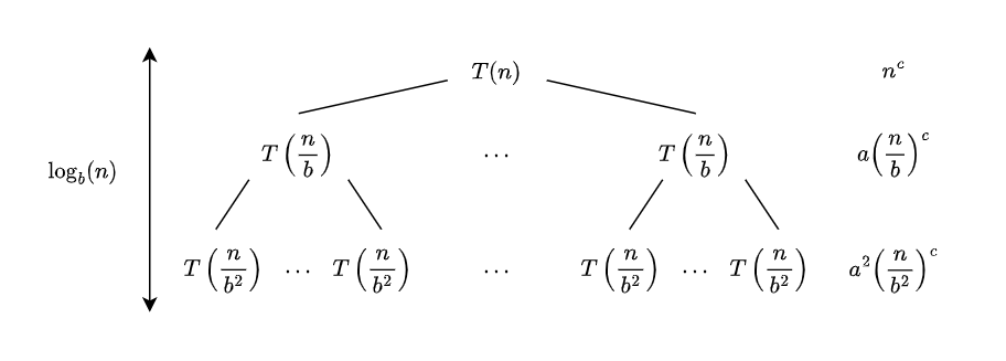
$T(n)$ has $a$ subtrees of size $\frac{n}{b}$, giving a complexity of $a\left(\frac{n}{b}\right)^c$ for the first level.
Each subtree in the first level has $a$ subtrees, giving a total of $a^2$ subtrees in the second level. Each of these contributes $\frac{n}{b^2}$ to the complexity, giving $a^2\left(\frac{n}{b^2}\right)^c$ for the second level.
From this, it can be seen that the complexity at level $i$ is given by $a^i\left(\frac{n}{b^i}\right)^c$, which can be rearranged to $\left(\frac{a}{b^c}\right)^i n^c$. The tree has height $\log_bn$, so the solution to the recurrence is given by $$ \begin{aligned} T(n) &\leq n^c \sum_{i=0}^{\log_bn}\left(\frac{a}{b^c}\right)^i\\ T(n) &= O\left(n^c \sum_{i=0}^{\log_bn}\left(\frac{a}{b^c}\right)^i\right) \end{aligned} $$
For case $c = \log_ba$
Rearranging $c = \log_ba$: $$ \begin{aligned} c &= \log_ba\\ log_b(b^c) &= \log_ba\\ b^c &= a \end{aligned} $$ Substituting this into the equation for $T(n)$ gives $$ T(n) = O\left(n^c \sum_{i=0}^{\log_bn}\left(1\right)^i\right) = O\left(n^c \left(\log_bn\right)\right) = O\left(n^c \log n\right) $$
For case $c > \log_ba$
Rearranging $c > \log_ba$ gives $a < b^c$. Because $\frac{a}{b^c} < 1$, the summation in $T(n)$ converges to a constant: $$ \sum_{i=0}^{\log_bn}\left(\frac{a}{b^c}\right)^i = O(1) $$ This gives $$ T(n) = O(n^c \times O(1)) = O(n^c) $$
For case $c < \log_ba$
Rearranging $c < \log_ba$ gives $b^c < a$, so $\frac{a}{b^c} > 1$. Using the sum of geometric series and some rules for logarithms, the summation can be expanded to $$ \begin{aligned} \sum_{i=0}^{\log_bn}\left(\frac{a}{b^c}\right)^i &= \frac{\frac{a}{b^c}^{1 + \log_bn}-1}{\frac{a}{b^c} - 1}\\ &= O\left(\frac{a}{b^c}^{1 + \log_bn}\right)\\ &= O\left(\frac{a}{b^c}\times \frac{a}{b^c}^{\log_bn}\right)\\ &= O\left(\frac{a}{b^c}^{\log_bn}\right)\\ &\text{using } x = y^{\log_yx} \text{:}\\ &= O\left(\frac{\left(b^{\log_ba}\right)^{\log_bn}}{\left(b^c\right)^{\log_bn}}\right)\\ &= O\left(\frac{\left(b^{\log_bn}\right)^{\log_ba}}{\left(b^{\log_bn}\right)^c}\right)\\ &= O\left(\frac{n^{\log_ba}}{n^c}\right) \end{aligned} $$ Therefore, $T(n)$ is given by $$ T(n) = O\left(n^c \times O\left(\frac{n^{\log_ba}}{n^c}\right)\right) = O\left(n^{\log_ba}\right) $$
Therefore all cases of the master theorem have been proven. $\blacksquare$
Dynamic programming
Dynamic programming, like divide and conquer, involves breaking a larger problem down into sub-problems recursively but instead of combining the results after recursion dynamic programming stores the solutions to sub-problems and these can later be used to solve other sub-problems or to obtain an optimal solution.
Dynamic programming algorithms covered:
Weighted Interval Scheduling
Input $n$ intervals $(s_i, f_i)$ with weight $v_i$
Output A compatible subset of intervals which maximises total weight
Suppose requests are sorted by ascending finish time, that is $f_1\leq f_2 \leq ... \leq f_n$. Let $p(j)$ be the largest index $i < j$ such that $i$ and $j$ are compatible and $p(j) = 0$ if there are no compatible intervals.
Consider the final interval, $n$. If this interval is included in an optimal solution then any intervals between $p(n)$ and $n$ are incompatible by definition of $p(n)$. The optimal solution therefore contains $n$ and some intervals from $\lbrace 1,...,p(n)\rbrace$.
If $n$ is not in the optimal solution then the optimal solution only contains intervals $\lbrace 1,...,n-1 \rbrace$. To maximise the total weight of the schedule, the maximum of these two options is taken, which results in a recursive definition as follows: $$ M[j] = \begin{cases} 0 & j=0\\ \max\left(M[j-1], M[p(j)]+v_j \right) & \text{if } j > 0 \end{cases} $$
This finds the maximum weight of a schedule up to an interval $j$. It considers the maximum of $M[j-1]$, which is the case where $j$ is not in the optimal solution and $M[p(j)] + v_j$, which is the case where the $j$ is in the optimal solution. By including the maximum weight at each stage, the final schedule weight is guaranteed to be maximum.
Complexity
Implementing the above recursively takes at worst exponential time. This can be improved to linear by using memoisation.
for i from 1 to n in intervals sorted by finish time:
    calculate M[i]
This takes $O(n)$ time, assuming the intervals are already sorted and $p(j)$ has been calculated for each interval. This is because addition, subtraction, $\max$ and lookup for $M$, $p$ and $v$ is $O(1)$, so over $n$ intervals the total time taken is $O(n)$.
Finding a solution
The above algorithm calculates the maximum value of a schedule, but does not give the schedule itself. The values calculated can be used to find the schedule.
$$ S[j] = \begin{cases} {j} \cup S[p(j)] & \text{if }M[j] > M[j-1]\\ S[j-1] & \text{otherwise} \end{cases} $$
Then
for i from 1 to n in intervals:
    calculate S[i]
The complexity of this algorithm is $O(n)$. The schedule of maximum weight is then given by $S[n]$.
Subset Sum
Input Positive integers $w_1, w_2, ..., w_n$ and an integer $W$
Output A subset of the integers whose sum is as large as possible, but less than $W$
[ADD DESCRIPTION OF SUBPROBLEMS]
$$ M[j, c] = \begin{cases} 0 & \text{if } w_j = 0 \text{ or } c = 0\\ M[j-1, c] & \text{if } w_j > c\\ \max(M[j-1, c], w_j + M[j-1, c-w_j]) & \text{if } w_j \leq c \end{cases} $$
Then
for j from 1 to n:
    for c from 0 to W:
        calculate M[j,c]
return M[n, W]
Complexity
$O(nW)$ time as seen above.
Sequence Alignment
Input Two finite words $x_1x_2...x_m$ and $y_1y_2...y_n$, the gap and mismatch penalties
Output The minimum cost alignment and its distance
The minimum edit distance or Levenshtein distance between two words is a measure of their similarity. Consider the word occurrence and the misspelling ocurrance. These could be aligned as follows:
o-currance
occurrence
where - indicates a gap. This distance between the two is a gap and one mismatch. They could also be aligned as
o-curr-ance
occurre-nce
which has three gaps and no mismatches. To determine which of these is better, there are different penalties for gaps and mismatches.
Let $\delta$ denote the gap penalty and $\alpha_{ab}$ denote the mismatch penalty for two letters $a$ and $b$.
A possible definition of $\alpha_{ab}$ is $$ \alpha_{ab} = \begin{cases} 0 & \text{if } a=b\\ 1 & \text{if } a \text{ and } b \text{ are both vowels or consonants}\\ 3 & \text{otherwise} \end{cases} $$
The cost of an alignment is therefore the minimum sum of gap and mismatch costs. The aim is to find the alignment of minimum cost between two words.
In an optimal alignment either
- the last letters of $x$ and $y$ are matched
- the last letter of $x$ is aligned with a gap
- the last letter of $y$ is aligned with a gap
As a recurrence, this is $$ D[i,j] = \begin{cases} j \times \delta & i = 0\\ i \times \delta & j = 0\\ \min(\alpha_{x_iy_i}+D[i-1, j-1], \delta + D[i-1, j], \delta + D[i, j-1]) & \text{if } i \geq 1 \text{ and } j \geq 1 \end{cases} $$
Then
for j from 1 to n:
    for i from 1 to m:
        calculate D[i,j]
return D[m,n]
This takes $O(mn)$ time.
Finding an alignment in linear space
[TODO]
Computational complexity
Computational complexity classifies algorithmic problems based on their relative hardness.
Topic covered:
Polynomial-time reductions
A polynomial time reduction from an algorithmic problem $X$ to another problem $Y$ is a polynomial algorithm for $X$ that uses $Y$, denoted $X \leq_p Y$. These calls to $Y$ are called oracle calls.
If $X \leq_p Y$ then
- There is a polynomial reduction from $X$ to $Y$
- $X$ can be reduced to $Y$
- $X$ is polynomial-time reducible to $Y$
- $Y$ is at least as hard as $X$
- If there is a polynomial time algorithm for $Y$ then there is a polynomial time algorithm for $X$
- If no polynomial-time algorithm exists for $X$ then no polynomial time algorithm exists for $Y$
Polynomial time reductions can be composed. If $X \leq_p Y$ and $Y \leq_p Z$ then $X \leq_p Z$.
For this module, reductions focus on decision problems. These are problems which can be answered with yes or no. For example, instead of "Find the shortest path from $u$ to $v$" a decision problem would be "Does there exists a path from $u$ to $v$ of length $k$?"
Independent set
An independent set of vertices is one in which no two vertices share an edge. More formally, an independent set is a set of vertices $S$ such that $S \subseteq V$ and $\forall v, w \in S$, $(v,w) \notin E$.
Consider the following graph
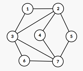
${3, 4, 5}$ is an independent set in the graph and ${1, 4, 5, 6}$ is the maximum independent set.
The independent set ($\text{IS}$) decision problem is as follows:
Input Undirected graph $G = (V, E)$ and a number $k$
Output Yes if $G$ has an independent set of size $k$, no otherwise
Vertex cover
A vertex cover is a set of vertices such that every edge is incident to some vertex in the set. More formally, a vertex cover is a set $S$ such that $S \subseteq V$ and $\forall (v,w) \in E$ either $v \in S$ or $w \in S$.
${1, 2, 6, 7}$ is a vertex cover in the graph above. ${2, 3, 7}$ is the minimum vertex cover.
The vertex cover ($\text{VC}$) decision problem is as follows:
Input Undirected graph $G = (V, E)$ and a number $k$
Output Yes if $G$ has a vertex cover of size $k$, no otherwise
Reductions
The largest independent set and smallest vertex cover partition the set of vertices. For the example above, ${1, 4, 5, 6} \cup {2, 3, 7} = V$.
$S$ is an independent set if $V \setminus S$ is a vertex cover.
Using this, independent set can be reduced to vertex cover in polynomial time, that is, $\text{IS} \leq_p \text{VC}$. The reduction is as follows:
$\text{IS}(G, k) = \text{VC}(G, |V| - k)$
This is a polynomial time reduction because
- it has polynomially many steps (in this case 1)
- makes oracle calls to $\text{VC}$
Vertex cover can also be reduced to independent set:
$\text{VC}(G, k) = \text{IS}(G, |V| - k)$
As the problems have been reduced in both directions, independent set and vertex cover are polynomially equivalent, denoted $\text{IS} \equiv_p \text{VC}$.
Set cover
A set cover of a set is a set of subsets which contain all items in the set. For example, ${1,2}, {3,4}$ would cover the set ${1,2,3,4}$.
The set cover ($\text{SC}$) decision problem is as follows:
Input Set of $U$ elements and a collection of subsets $S_1, S_2, ..., S_n \subseteq U$
Output Yes if there is a collection of subsets of size $k$ which cover the set, no otherwise
Vertex cover can be reduced to set cover. Let $I_v$ be the set of edges incident to a vertex $v$, that is, $I_v = {e \in E ;:; v \in e}$. The set cover of these edges of size $k$ is exactly the same as the vertex cover of size $k$, so the reduction is
$\text{VC}(G, k) = \text{SC}(E, {I_v ;:; v \in V}, k)$ where $G = (V, E)$.
Boolean satisfiability
A Boolean expression is satisfiable if there is some assignment of variables such that the expression evaluates to true.
The $\text{SAT}$ decision problem is as follows:
Input Boolean expression in conjunctive normal form (CNF) over a set of variables $x_1, ..., x_n$
Output Yes the expression is satisfiable, no otherwise
A CNF expression consists of a conjunction (and) of disjunctions (or), such as $(x_1 \vee x_2 \vee x_3) \wedge (x_4 \vee x_5) \wedge (\bar{x}_1 \vee \bar{x}_4)$.
A literal is a variable or its negation, such as $x_1$ and $\bar{x}_1$. A clause is a disjunction of literals, such as $(x_4 \vee x_5)$.
$\text{3-SAT}$ is a variation of $\text{SAT}$ with at most 3 literals per clause.
Consider the $\text{3-SAT}$ instance $(\bar{x}_1 \vee x_2 \vee x_3) \wedge (\bar{x}_2 \vee x_1 \vee x_3) \wedge (\bar{x}_1 \vee x_2 \vee x_4)$. $\text{3-SAT}$ can be reduced to $\text{IS}$ by producing a graph $G = (V, E)$ where $V$ is every literal occurrence ($x_1$ and $\bar{x}_1$ are distinct literal occurrences) and $E$ contains an edge between every literal in the same clause and between pairs of negated literal occurrences.
For example, the instance above becomes
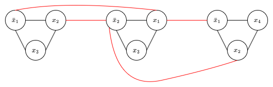
where the black edges are between literal occurrences in the same clause and red edges are between literal occurrences and their negations in different clauses.
Only one literal occurrence in each clause needs to be satisfied to satisfy the expression. A clause is represented by a triangle in the graph. That means there must be an independent set with one vertex in each triangle, so $\text{3-SAT}$ can be reduced to $\text{IS}$.
$\text{3-SAT}(\phi) = \text{IS}(G_\phi, k)$ where $G_\phi$ is the graph as obtained from the $\text{3-SAT}$ instance $\phi$ as above and $k$ is the number of clauses in $\phi$. Because the graph can be constructed in polynomial time, this is a polynomial time reduction. $\text{3-SAT} \leq_p \text{IS}$.
P and NP
[add some more stuff here]
Suppose $Z$ in NP-complete. If $X \in \text{NP}$ and $Z \leq_p X$ then $X$ is NP-complete.
NP-completeness
CS261 - Software Engineering
Methodologies
- Plan-driven - all of the process activities are planned in advance, progress is measured against initial plan, fixed specification before development starts
- Agile - Incremental planning, more adaptable
Most methodologies consist of design, implementation, testing and maintenance.
Waterfall model
The waterfall model is an example of plan-driven development.
- Linear ordering of processes
- Each stage must be completed before moving on to the next
- Allows distributed development
The waterfall model is ideal for projects where the requirements are understood and will not change. It allows each component to be tested independently and it's easy to add members to a team because the whole system is well documented.
The waterfall model is not adaptable and the customer will have to wait a long time to see results. It is difficult to respond to changing customer requirements. This means it is not ideal for long term projects.
Incremental development
More flexible than waterfall but still plan-driven, software can be developed in stages with customer feedback incorporated between iterations.
Advantages
- The cost of accommodating changing customer requirements is reduced
- Software is available to the customer quicker which allows for quicker feedback
- Greater perceived value for money
- Includes user acceptance testing in each stage
Disadvantages
- Difficult to estimate the cost of development
- Difficult to maintain consistency with new features being added
- Harder to include new features or make changes to fundamental components
- Not cost effective to produce documentation for every version of the software
- Increased cost of repeated deployment
Reuse-oriented software
Rewriting software from scratch is unnecessary and expensive so development can rely on a large base of reusable components instead.
Software specification
Software specification is the first stage of a software methodology. It requires understanding and definition of required services in a system and identification of constraints. This process is also called requirements engineering and results in a requirements document. This document has to be understood by both the customer and developers. Requirements engineering is divided into 4 steps.
- Feasibility study - Determine that the task is feasible and cost-effective
- Requirements elicitation and analysis - Derive the system requirements from the customer
- Requirements specification - Translate information from the previous stage into formal documents that define the set of requirements
- Requirements validation - Ensure the requirements are achievable and valid These four stages come together to form the requirements document.
Agile development
Principles of agile development
- Customer involvement - The customer can provide and prioritise new system requirements and evaluate iterations
- Incremental delivery - Software is developed in increments with the customer specifying the requirements for the next iteration
- People, not processes - Skills of the development team should be recognised, team members should develop their own ways of working
- Embrace change - Design a system that accommodates change
- Maintain simplicity - Focus on simplicity in the software being developed
Agile focuses more on development than documentation so it can be harder to make changes later. This can also cause problems if the team changes.
Extreme programming
- Extreme programming is an agile method with incremental delivery and fast iterations
- Versions will be built several times a day and delivered to the customer every few weeks
- Automated tests are used to verify builds and builds are only accepted if all tests pass
- Code is continually refactored to maintain simplicity
- Strong customer involvement
- Simple design
- Test-driven development - tests are written before the software
- Pair programming - developers work in pairs checking each others work and providing support
- Collective ownership - pair programming means at least two people understand it
- Continuous integration - components are integrated as soon as they are ready
- Sustainable pace
- On-site customer - easier to get feedback
Scrum
Scrum is an agile method which focuses on managing iterative development it has 3 primary phases
- Outline planning phase - establish general goals
- Sprint cycles - each cycle develops an increment of the system
- Project closure - wrap up the project, document and deliver
A scrum master interfaces between the developers and customer.
Prototypes or MVPs
Prototypes are for testing feasibility and proof of concept and presenting to customers. They are not necessarily a complete solution.
Minimum Viable Products (MVPs) meet the fundamental requirements for deployment to production. They are mostly finished products.
Requirements analysis
Requirements are descriptions of what the system should do, the service it provides and the constraints on its operation. They provide a basis for tests, validation and verification and enable more accurate cost estimation.
Requirements are a bridge between customers and developers, so requirements need to be specified so both the customer and developers can understand them. There is a notion of C- and D-facing requirements, written to be understood by the customer and developers respectively.
Customer requirements (C-facing) define how the system should work from the user's view. They use natural language and diagrams. Developer requirements (D-facing) use detailed, technical descriptions and define exactly what must be designed and implemented.
Requirements describe what needs to be built, whereas design and implementation are how it is built.
Requirements should be
- Prioritised - Must/should/could/won't
- Consistent - requirements don't conflict
- Modifiable - requirements can be changed
- Traceable - each requirement should have a reason
- Correct - a requirement should accurately describe its functionality
- Feasible
- Necessary
- Unambiguous
- Verifiable - can be tested
The requirements analysis document needs to be understood by customers, managers, engineers, testers and maintainers.
The requirements analysis document consists of a preface, introduction, glossary, user requirements design (customer facing requirements), system architecture (high level overview of system), system requirements specification (functional and non-functional requirements), system models (relationships between components), system evolution and appendices.
Functional requirements describe what the system should do. Non-functional requirements describe qualities of a system such as availability, performance and deployment. They specify constraints on the system and legal constraints.
Requirements elicitation and analysis consists of a few stages
- Discovery - interview stakeholders
- Classification - categorise discovered requirements
- Prioritisation and negotiation - prioritise requirements and negotiate conflicting requirements
- Specification - Put the requirements in a document for stakeholders to review, then repeat the process if more changes have to be made
Requirements need to be validated.
- Validity - will the system support the customer's needs?
- Consistency - are there any conflicts?
- Realism - can the system be produced with available technologies and resources?
- Verifiability - Once complete, can the system be shown to satisfy the requirements?
Requirements must take into consideration legal, social and professional issues including respecting copyright and patents, recognising developers, not breaking any laws and working in the best interest of the 🅱ustomer.
Project management
A project may fail if the requirement specification was poor, deadlines were unrealistic, budget was insufficient, communication was poor, testing was inadequate or team members did not fulfil their tasks.
The four main goals of project management are
- Deliver the software at the agreed time
- Keep overall costs within budget
- Deliver software that meets the customers expectations
- Maintain a happy and well-functioning development team
The success of a team depends on three generic factors
- The people in the team
- The group organisation
- Technical and managerial communications
Risk management
Steps for risk management
- Identify
- Analyse
- Plan
- Monitor
Risks can be grouped by what they affect. Project risks affect the project schedule or resources. Product risks sre those that affect the quality or performance of the software being developed. Business risks are those that affect the organisation developing the software.
Project planning
Project managers must break down the work into parts and assign each part to a team member. They must also anticipate and deal with problems which may arise. Project planning takes place in 3 stages:
- Proposal stage
- Startup phase
- Periodical planning
Project scheduling involves identifying activities, estimating resources and allocating activities to people. Gantt charts can be used to represent project schedules.
Schedule estimation can be done based on past experience or using an algorithm to estimate based on project attributes.
A project is successful if it meets the original specification and the customer's expectations.
System design
System design is supported by system modelling.
System modelling perspectives:
- External - model the context of the system
- Interaction - model the interactions between the system and its environment, or between components of a system
- Behavioural - model dynamic behaviour of the system
- Structural - model the organisation of a system or the structure of the data being processed
System modelling encourages ambiguity resolution.
UML is a modelling language to represent static and dynamic parts of the system. Creating static views of a system requires identifying entities (objects).
A class diagram in UML shows entities and their relationships. It gives the class name, attributes and methods. + and - denote public and private methods respectively. They do not include setters, getters and inherited methods. Static attributes/methods should be underlined. Abstract class names are styled in italics and interfaces are surrounded with << >>.
Arrows between classes denote parent-child relationships. Arrows go from child to parent. A solid line with black arrow denotes a class, a solid line with white arrow denotes an abstract class and a dashed line with a white arrow denoted an interface.
Entities in a class diagram can be linked together to represent relationships. These associations have several features
- Multiplicity -
a..bmeans betweenaandbinclusive, whereaandbare numbers. Ifbis omitted it means "aor more".*denotes zero or more. - Name - what relationship the objects have, such as "contains" or "creates"
- Navigability - direction
Entities can have one-to-one or one-to-many relationships.
A white diamond denotes aggregation and means one class in part of the other, like an engine being part of a car. A black diamond denotes composition and means one class is made up of the other, like a book is made up of pages. The book entity cannot exist without the page entity, whereas the car can without the engine so composition is stronger than aggregation. A dashed line denotes temporary dependency.
For example, a diagram may contain cinema, movie and box office as entities with a black diamond from box office to cinema and a white diamond from movie to cinema. If the cinema is destroyed, so is the box office (composition) but the movies will still exists (aggregation).
Context models illustrate the operational context of the system and other systems.
Structural models show the organisation of components in a system. UML diagrams are an example of these.
Activity diagrams are used to represent workflows of stepwise activities, like a flowchart.
Interaction models show user interaction with the system. In UML these are use case diagrams and sequence diagrams. A use case diagram represents a user's interactions with the system and a sequence diagram shows a user's interactions over time.
A state machine diagram is a finite state machine showing how the state of the system changes, like an NFA but less CS259-y.
Architectural design
Architectural design is concerned with understanding how a system should be organised. Some common architectural patterns include
- Layered - structure system into layers that provide services to the layer above, each layer only relies on the layer below it. Good for modular design but may not be an ideal structure for some systems
- Repository - all data is in a central repository and all interaction is done through it. Efficient for sharing data but introduces a single point of failure
- Pipe and filter - Components take data, transform it and then pipe it to other components. Components can be reused, flexible but requires standardised data format. Ideal for batch processing
- Model-View-Controller (MVC) - focusses on how to interpret user interactions, update data and present that to the user. Provides separation between presentation, interaction and data but can make design more complex. Ideal for UI
Implementation
Design patterns can be used to solve common programming problems. Encapsulation, inheritance, iteration and exceptions are design patterns.
Creational patterns are design patterns for creating objects.
- Factories - method which produces classes of a particular type
- Builders - objects created step by step using methods
- Prototypes - clone objects to make new objects
Structural patterns are used to realise relationships between entities.
- Proxy - Stand in for another object, can load the original when needed
- Decorator - Adds new behaviour to objects at runtime
- Adaptor - Allows output from one object to be used by another
- Flyweight - Store one copy of expensive attributes in a static class and reference it
Behavioural patterns are concerned with how objects communicate.
- Iterator - Traverse a container to access its elements
- Observer - Notifies other objects if state changes are made
- Memento - Save and restore objects without revealing its implementation details
- Strategy - Select the method to complete a task at runtime
Design patterns help achieve the SOLID design principles.
- Single responsibility - a class should be responsible for a single piece of functionality
- Open/closed - once designed and completed, a class should be extended, not modified
- Liskov substitution - an object that uses a parent class can use its child classes without knowing
- Interface segregation - Many specific interfaces are better than a general one
- Dependency inversion - high level classes don't depend on low level classes
Human computer interaction
HCI is the study of how humans interact with computers. There are four main human traits that underpin HCI.
-
Attention
- Selective attention - tune other things out to focus on a particular set of stimuli
- Divided attention - focussing on multiple things at once
- Sustained attention - attention span
- Executive attention - more organised attention
-
Memory
- Sensory stores - visual and auditory stores hold information before it enters working memory
- Working memory - Holds transitory information and makes it available for further processing
- Long-term memory
-
Cognition - the process by which we gain knowledge
Norman's human action cycle is the idea that humans go through a cycle of 7 stages when interacting with a computer system.
- Form a goal
- Intention to act
- Planning to act
- Execution
- Feedback
- Interpret feedback
- Evaluate outcome
The human action cycle is used to evaluate the effectiveness of a user interface. It focusses on two particular aspects, the gulf of evaluation and the gulf of execution. The gulf of evaluation is the psychological gap which must be crossed to interpret a UI. The gulf of execution is the gap between the user's goals and the means to execute these goals. Both of these gulfs need to be minimised.
The Gestalt laws of perceptual organisation are a set of principles around human visual perception.
- Figure ground principle - People tend to segment their vision into the figure and the ground, the figure is the focus and the ground is the background.
- Similarity principle - If two things look similar, they should behave the same way
- Proximity principle - If objects are close together they must be related
- Common region principle - If objects in the same closed region (like a border) are grouped together
- Continuity principle - If objects are in a line or a curve they are perceived as related
- Closure principle - If there is a complex arrangement of shapes they are perceived as a single pattern
- Focal point principle - People are drawn to the most unique part of an image
-
Affordances - what an object allows us to do, a door affords opening it. It is important to make affordances as clear as possible. Signifiers are cues about an object's affordances.
Nielson's Usability Principles
- Visibility of system status
- Match between system and real world
- User control and freedom
- Consistency and standards
- Help users recognise and recover from errors
- Error prevention
- Recognition rather than recall
- Flexibility and efficiency of use
- Aesthetic and minimalist design
- Help and documentation
Software dependability
Software systems need to be dependable. If they are not, people won't use them.
Reliability is a measure of how likely the system is to provide its service for some amount of time. Perceived reliability is how reliable the system appears to the user.
Reliability can be measured using
- Probability of failure on demand
- Rate of occurrence of failures
- Mean time to failure
- Availability
There are many attributes of a dependable system
- Availability
- Reliability
- Safety
- Confidentiality
- Integrity
- Maintainability
A fault is the cause of an error. A failure is the result of an error propagating beyond a system boundary.
Some causes of system failures include
- Hardware failure
- Software failure
- Operational failure
Dependability can be proved using
- fault avoidance
- fault detection and correction
- fault tolerance
Graceful degradation means the system is able to operate, possibly with reduced capacity, in the event of component failure. Redundancy is spare capacity included in a system that can be used in case of a failure. If components are diverse they are less likely to fail in the same way.
Dependable processes are those that produce dependable software. Dependable processes are
- Documentable
- Standardised
- Auditable
- Diverse
- Robust
System architectures also need to be dependable. This can be achieved with
- Protection systems
- Self-monitoring architectures
- N-version programming
- Software diversity
System testing
Testing shows a program does what it was intended to do. It highlights defects before the software is in use.
Static testing is testing without execution. Dynamic testing is executing test cases.
- Structural/white-box testing are test cases derived from control/data flow of system
- Functional/black-box testing are test cases derived from formal component specification
Statement adequacy means all statements have been executed by at least one test. Statement coverage is number of executed statements divided by number of statements.
Unit tests test the simplest parts of a system, like objects and methods. Component or integration testing tests how units interact with each other.
Test driven development develops tests before writing code and development does not continue until all tests pass.
User testing ensures the system works in a variety of environments.
- Alpha testing - small group, early release
- Beta testing - larger group, later release
- Acceptance testing - larger group, final system
Release management
Version control manages code changes over time and allows rolling back to previous versions.
Systems can be released into different environments during release, such as test, development, feature and master.
CS262 - Logic and Verification
Propositional logic is a formal system for reasoning about propositions. A proposition may also be called a statement or formula. Atomic propositions can not be split. Atomic propositions can be joined using logical connectives to form new propositions. Common connectives include $\neg$, $\wedge$, $\vee$ and $\rightarrow$. Binary connective can generally be denoted using $\circ$. For example, $\circ = \{\wedge, \vee, \rightarrow, ...\}$.
Atomic formulae include propositional variables and $\top$ or $\bot$. If $X$ is a formula so is $\neg X$. If $X$ and $Y$ are formulae then so is $X \circ Y$.
A parse tree can be constructed for any propositional formula. An atomic formula $X$ has a single node labelled $X$. The subtree for $\neg X$ has a node labelled $\neg$ with the subtree $X$ as a child. The parse tree for $X \circ Y$ has a node labelled $\circ$ as the root and the parse trees for $X$ and $Y$ as left and right subtrees respectively.
In propositional logic, formulae can have one of two possible values, T or F. A truth table lists each possible combination of truth values for the variables of a Boolean function.
A valuation is a mapping $v$ from the set of propositional formula to the set of truth values satisfying the following conditions:
- $v(T) = T$, $v(F) = F$
- $v(\neg X) = \neg v(X)$
- $v(X \circ Y) = v(X) \circ v(Y)$
The truth table of a formula lists all possible valuations.
A formula that evaluates to T under all valuations is a tautology. A formula that evaluated to F under all valuations is a contradiction. A formula that evaluates to T for some valuation is called satisfiable.
A formula $X$ is a consequence of a set $S$ of formulae, denoted $S \vDash X$, provided $X$ maps to T under every valuation that maps every member of $S$ to T. $X$ is a tautology if and only if $\emptyset \vDash X$, which is written as $\vDash X$. More simply, $S$ is the set of formulae which need to be true for $X$ to be true.
Formulae representing the same truth function are called logically equivalent. $p \rightarrow q = \neg p \vee q$.
Normal forms
A set of connectives is said to be complete if we can represent every truth function $\{T,F\}^n \rightarrow \{T, F\}$ using only these connectives.
Consider a function $f$ on variables $x_1, ..., x_n$. For the values $v_i$ where $f(v_1, ..., v_n) = T$, if $v_i$ is T then replace it with $x_i$ or $\neg x_i$ if $v_i$ is F and take the conjunction. Then take the disjunction of these conjunctions. This shows that $\{\wedge, \vee, \neg\}$ is complete as any formula can be expressed using only these connectives. The resulting formula is said to be in disjunctive normal form (DNF). The DNF of a function of not unique.
A literal is a variable, its negation, $\bot$ or $\top$.
DNF is the disjunction of conjunctions of literals.
Conjunctive normal form (CNF) is the conjunction of disjunctions of literals.
Every Boolean function has a CNF and DNF.
Let $X_1, X_2, ..., X_n$ be a sequence of propositional formulas.
A generalised disjunction is written as $[X_1,X_2,...,X_n] = X_1 \vee X_2 \vee ... \vee X_n$.
A generalised conjunction is written as $\left<X_1, X_2, ..., X_n\right> = X_1 \wedge X_2 \wedge ... \wedge X_n$.
If $X_1, ... X_n$ are literals then $[X_1, ...]$ is a clause and $\left< X_1, ...\right>$ is a dual clause.
$v([]) = F$ and $v(\left<\right>) = T$. These are the neutral element of disjunction and conjunction respectively.
$\alpha$ and $\beta$ formulae
All propositional formulae of the forms $X \circ Y$ and $\neg(X \circ Y)$ are grouped into two categories, those that act conjunctively and those that act disjunctively.
The below tables can be derived from the following definitions:
- $\alpha = \alpha_1 \wedge \alpha_2$
- $\beta = \beta_1 \vee \beta_2$
Conjunctive
| $\alpha$ | $\alpha_1$ | $\alpha_2$ |
|---|---|---|
| $X \wedge Y$ | $X$ | $Y$ |
| $\neg(X \vee Y)$ | $\neg X$ | $\neg Y$ |
| $\neg(X \rightarrow Y)$ | $X$ | $\neg Y$ |
| $\neg(X \leftarrow Y)$ | $\neg X$ | $Y$ |
| $\neg(X \uparrow Y)$ | $X$ | $Y$ |
| $X \downarrow Y$ | $\neg X$ | $\neg Y$ |
| $X \not\rightarrow Y$ | $X$ | $\neg Y$ |
| $X \not\leftarrow Y$ | $\neg X$ | $Y$ |
Disjunctive
| $\beta$ | $\beta_1$ | $\beta_2$ |
|---|---|---|
| $\neg(X \wedge Y)$ | $\neg X$ | $\neg Y$ |
| $X \vee Y$ | $X$ | $Y$ |
| $X \rightarrow Y$ | $\neg X$ | $Y$ |
| $X \leftarrow Y$ | $X$ | $\neg Y$ |
| $X \uparrow Y$ | $\neg X$ | $\neg Y$ |
| $\neg(X \downarrow Y)$ | $X$ | $Y$ |
| $\neg(X \not\rightarrow Y)$ | $\neg X$ | $Y$ |
| $\neg(X \not\leftarrow Y)$ | $X$ | $\neg Y$ |
For every $\alpha$- and $\beta$-formula valuation
- $v(\alpha) = v(\alpha_1) \wedge v(\alpha_2)$
- $v(\beta) = v(\beta_1) \vee v(\beta_2)$
CNF algorithm
Given any propositional formula, find $\left<\left[X\right]\right>$, which will give a conjunction of disjunctions of the form $\left<D_1, ..., D_n\right>$. Select one of these disjunctions which is not a disjunction of literals, and denote it $D_i$. Select a non-literal $N$ from $D_i$.
- If $N = \neg \top$ then replace $N$ with $\bot$
- If $N = \neg \bot$ then replace $N$ with $\top$
- If $N = \neg \neg Z$ then replace $N$ with $Z$
- If $N$ is a $\beta$-formula then replace $N$ with $\beta_1 \vee \beta_2$ (this is called $\beta$-expansion)
- If $N$ is a $\alpha$-formula then replace $D_i$ with two disjunctions, one in which $N$ is replaced with $\alpha_1$ and one in which $N$ is replaced by $\alpha_2$.
Example
$\neg(p\wedge \neg \bot) \vee \neg(\top \uparrow q)$
- Take conjunction of disjunction: $\left<\left[\neg(p\wedge \neg \bot) \vee \neg(\top \uparrow q)\right]\right>$
- Apply $\beta$ expansion: $\left<\left[\neg(p\wedge \neg \bot), \neg(\top \uparrow q)\right]\right>$
- Apply $\beta$ expansion: $\left<\left[\neg p, \neg \neg \bot, \neg(\top \uparrow q)\right]\right>$
- Apply double negation: $\left<\left[\neg p, \bot, \neg(\top \uparrow q)\right]\right>$
- Apply $\alpha$ expansion: $\left<\left[\neg p, \bot, \top\right], \left[\neg p, \bot, q\right]\right>$
- Formula is now in CNF, stop.
Correctness of the algorithm
The algorithm produces a sequence of logically equivalent formulas.
The proof for $\beta$-expansion is trivial. $\alpha$-expansion can be demonstrated by distributivity: $D_i = [\alpha, X_2, ...,X_k]$ is equivalent to $(\alpha_1 \wedge \alpha_2) \vee (X_2 \vee ... \vee X_k)$ which by distributivity is $(\alpha_1 \vee (X_2 \vee ... \vee X_k)) \wedge (\alpha_2 \vee (X_2 \vee ... \vee X_k))$ which, by associativity, can be written as $\left<\left[\alpha_1, X_2, ..., X_k\right], \left[\alpha_2, X_2, ..., X_k\right]\right>$
The algorithm terminates, regardless of which choices are made during the algorithm.
Consider a rooted tree. A branch is a sequence of nodes starting at the root and finishing at a leaf. A tree is finitely branching if every node has finitely many children. A tree/branch is finite if it has a finite number of nodes.
König's lemma states that a tree that is finitely branching but infinite must have an infinite branch.
The rank, $r$, of a propositional formula is defined as follows
- $r(p) = r(\neg p) = 0$ for variables $p$
- $r(\top) = r(\bot) = 0$
- $r(\neg \top) = r(\neg \bot) = 1$
- $r(\neg \neg Z) = r(Z) + 1$
- $r(\alpha) = r(\alpha_1) + r(\alpha_2) + 1$
- $r(\beta) = r(\beta_1) + r(\beta_2) + 1$
- $r\left(\left[X_1, ..., X_n\right]\right) = \sum^n_{i=1}r(X_1)$
Example
$r((m \rightarrow \neg n) \wedge (\neg \neg o \wedge \neg \bot))$
- $r(m) = r(\neg m) = r(\neg n) = 0$
- $r(\neg \neg o) = r(o) + 1 = 0 + 1 = 1$
- $r(\neg \bot) = 1$
- $r(m \rightarrow \neg n) = r(\neg m) + r(\neg n) + 1 = 0 + 0 + 1 = 1$
- $r(\neg \neg o \wedge \neg \bot) = r(\neg \neg o) + r(\neg \bot) + 1 = 1 + 1 + 1 = 3$
- $r((m \rightarrow \neg n) \wedge (\neg \neg o \wedge \neg \bot)) = r(m \rightarrow \neg n) + r(\neg \neg o \wedge \neg \bot) + 1 = 1 + 3 + 1 = 5$
so the rank of the formula is 5.
A CNF expression is of the form $\left<\left[D_1, ..., D_n\right]\right>$. Each $D_i$ can be assigned a rank. Every step in the CNF algorithm decreases the rank of the disjunction or replaces it with two disjunctions of lower rank (in the case of $\alpha$-expansion). Consider each of the 5 rules of the CNF algorithm:
- Negation of $\top$ and $\bot$ will reduce rank from 1 to 0
- Double negation will reduce rank by 1
- $r(\alpha) = r(\alpha_1) + r(\alpha_2) + 1$, so $r(\alpha_1)$ and $r(\alpha_2)$ are both less than $r(\alpha)$. Therefore the two replacement disjunctions must each have lower rank.
- $r(\beta) = r(\beta_1) + r(\beta_2) + 1$ so the new disjunction has lower rank.
Given the above, an infinite branch is not possible, so the algorithm must terminate by König's theorem.
DNF algorithm
The DNF algorithm works very similarly to CNF. It starts by finding $\left[\left<X\right>\right]$. The first 3 rules are the same, but $\alpha$-expansion replaces a conjunction with $\alpha_1, \alpha_2$ and $\beta$-expansion replaces a conjunction with $\left[\left<..., \beta_1, ...\right>,\left<..., \beta_2, ...\right>\right]$, the opposite to the rules for a CNF.
Example
$\neg(p\wedge \neg \bot) \vee \neg(\top \uparrow q)$
- Take the disjunction of conjunctions: $\left[\left<\neg(p\wedge \neg \bot) \vee \neg(\top \uparrow q)\right>\right]$
- Apply $\beta$-expansion: $\left[\left<\neg(p\wedge \neg \bot)\right>,\left<\neg(\top \uparrow q)\right>\right]$
- Apply $\alpha$-expansion: $\left[\left<\neg(p\wedge \neg \bot)\right>,\left<\top, q\right>\right]$
- Apply $\beta$-expansion: $\left[\left<\neg p\right>, \left<\neg \neg \bot \right>, \left<\top, q\right>\right]$
- Apply double negation: $\left[\left<\neg p\right>, \left<\bot \right>, \left<\top, q\right>\right]$
- Formula is now in DNF, stop
Semantic tableau
There are two proof procedures for propositional logic - semantic tableau and resolution, closely connected to DNF and CNF respectively.
Both are refutation systems - to prove that a formula $X$ is a tautology, it begins with $\neg X$ and finds a contradiction.
Semantic tableau takes the form of a binary tree with nodes labelled with propositional formulae. Each branch can be seen as a conjunction of formulae on that branch and the tree is a disjunctions of all of its branches, hence DNF.
The tableau (tree) can be expanded. Select a branch and a non-literal formula $N$ on the branch
- If $N = \neg\top$ then extend the branch by a node labelled $\bot$ at its end
- If $N = \neg \bot$ then extend the branch by a node labelled $\top$ at its end
- If $N = \neg \neg Z$ then extend the branch by a node labelled $Z$ at its end
- If $N$ is an $\alpha$-formula, extend the branch by two nodes labelled $\alpha_1$, $\alpha_2$ ($\alpha$-expansion) at its end
- If $N$ is a $\beta$-formula, add a left and right child to the final node of the branch, labelled $\beta_1$ and $\beta_2$ ($\beta$-expansion)
Example
$\neg((p \rightarrow (q \rightarrow r)) \rightarrow ((p \vee s) \rightarrow ((q \rightarrow r) \vee s)))$
The following tree shows a partial expansion of the formula:
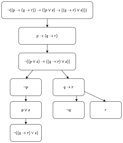
The formula is the root node. This is then $\alpha$-expanded to give two nodes. $p \rightarrow (q \rightarrow r)$ is then $\beta$-expanded to give a $\neg p$ and $q \rightarrow r$ as children at the end of the branch. $q \rightarrow r$ is $\beta$-expanded to give two literal children. $\neg((p \vee s)...)$ is $\alpha$-expanded to the two nodes at the end of the left branch.
A branch of a tableau is closed if both $X$ and $\neg X$ occur on the branch for some formula $X$ or if $\bot$ occurs on the branch. If $x$ and $\neg x$ appear on a branch then the branch is atomically closed. A tableau is (atomically) closed if every branch is (atomically) closed. A tableau proof for $X$ is a closed tableau for $\neg X$. If $X$ has a tableau proof this can be denoted $\vdash_t X$.
Example
$X = (p \wedge (q \rightarrow (r \vee s))) \rightarrow (p \vee q)$
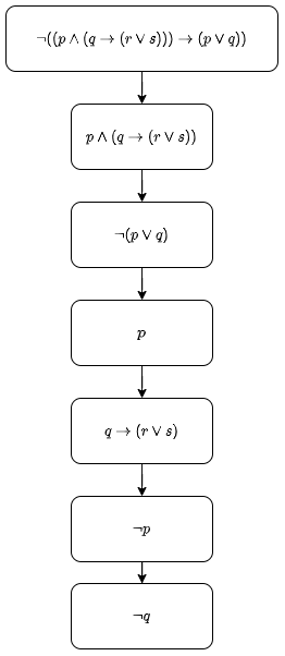
The above is closed because $p$ and $\neg p$ appear on the same branch. As this is the only branch the tableau is closed, meaning $X$ is a tautology.
A tableau is strict is no formula has had an expansion rule applied to it twice on the same branch.
To implement semantic tableau, the tree can be represented as a list of lists (disjunction of conjunctions). The strictness rule allows an expanded formula to be removed from a list. This is the same method as DNF expansion but it stops when a contradiction is found instead of continuing to literals.
The tableau proof system is sound - if $X$ has a tableau proof then $X$ is a tautology. This is proven by the correctness of DNF.
The tableau proof system is complete - if $X$ is a tautology then the strict tableau system will terminate with a proof for it.
Resolution proofs
Resolution proofs are closely linked to CNF expansion. Unlike semantic tableau, resolution proofs don't use a tree, they use $\left<\left[\dots\right],\dots,\left[\dots\right]\right>$ notation.
Like semantic tableau, resolution proof begins with the negation of the expression to prove.
In each step, select a disjunction and a non-literal formula $N$ in it
- If $N = \neg \top$, append a new disjunction where $N$ is replaced by $\bot$
- If $N = \neg \bot$, append a new disjunction where $N$ is replaced by $\top$
- If $N = \neg \neg Z$, append a new disjunction where $N$ is replaced by $Z$.
- If $N$ is an $\alpha$-formula, append two new disjunctions, one in which $N$ is replaced by $\alpha_1$ and another in which it is replaced by $\alpha_2$
- If $N$ is a $\beta$-formula, append a new disjunction where $N$ is replaced by $\beta_1, \beta_2$
A sequence of resolution expansion applications is strict if every disjunction has at most one resolution expansion rule applied to it. More simply, each disjunction can only be expanded once.
Resolution can be implemented using lists of disjunctions. Using the strict version means formulae can be removed from the list after having been expanded.
A resolution proof is closed if the empty clause, $\left[\;\right]$ appears in the list of disjunctions. This is because $v([\;]) = \bot$ and conjunction with $\bot$ will always be false. DNF expansion does not result in empty clauses, so the resolution rule is used.
The resolution rule is as follows: Suppose $D_1$ and $D_2$ are two disjunctions, with $X$ occurring in $D_1$ and $\neg X$ occurring in $D_2$. Let $D$ be the result of the following:
- delete all occurrences of $X$ from $D_1$
- delete all occurrences of $\neg X$ from $D_2$
- combine the resulting disjunctions
If a disjunction contains $\bot$, delete all occurrences of $\bot$ and call the resulting disjunction the trivial resolvent.
$D$ is the result of resolving $D_1$ and $D_2$ on $X$. $D$ is the resolvent of $D_1$ and $D_2$ and $X$ is the formula being resolved on. If $X$ is atomic, it is the atomic application of the resolution rule.
The resolution rule works because $\left<\left[X, Y\right],\left[\neg X, Z \right]\right> = \left<\left[X, Y\right], \left[\neg X, Z\right], \left[Y, Z\right]\right>$.
A resolution proof for $X$ is a closed resolution expansion for $\neg X$. If $X$ has a resolution proof this can be denoted $\vdash_r X$.
Example Resolution proof for $((p \wedge q) \vee (r \rightarrow s)) \rightarrow ((p \vee (r \rightarrow s)) \wedge (q \vee (r \rightarrow s)))$
- Take negation: $\left[\neg(((p \wedge q) \vee (r \rightarrow s)) \rightarrow ((p \vee (r \rightarrow s)) \wedge (q \vee (r \rightarrow s))))\right]$
- $\alpha$-expansion on 1: $\left[(p \wedge q) \vee (r \rightarrow s)\right]$ and $\left[\neg((p \vee (r \rightarrow s)) \wedge (q \vee (r \rightarrow s)))\right]$
- $\beta$-expansion on 2a: $\left[p \wedge q, r \rightarrow s\right]$
- $\beta$-expansion on 2b: $\left[\neg(p \vee (r \rightarrow s)), \neg (q \vee (r \rightarrow s))\right]$
- $\alpha$-expansion on 3: $\left[p, r \rightarrow s\right]$ and $\left[q, r \rightarrow s\right]$
- $\alpha$-expansion on 4: $\left[\neg p, \neg (q \vee (r \rightarrow s))\right]$ and $\left[\neg(r \rightarrow s), \neg (q \vee (r \rightarrow s))\right]$
- $\alpha$-expansion on 6a: $\left[\neg p, \neg q\right]$ and $\left[\neg p, \neg(r \rightarrow s)\right]$
- $\alpha$-expansion on 6b: $\left[\neg(r \rightarrow s), \neg q\right]$ and $\left[\neg(r \rightarrow s), \neg (r \rightarrow s)\right]$
- Resolution rule on $q$ for 5a and 7a: $\left[r \rightarrow s, \neg p\right]$
- Resolution rule on $p$ for 5a and 9: $\left[r \rightarrow s, r \rightarrow s\right]$
- Resolution rule on $r \rightarrow s$ for 8b and 10: $\left[\;\right]$
The empty clause creates a contradiction, meaning the original formula was a tautology.
Resolution properties
- The resolution method extends to first order logic (quantifiers).
- Resolution can also be generalised to establish propositional consequences.
- Resolution rules are non-deterministic
The resolution proof system is sound. If $X$ has a resolution proof then $X$ is a tautology.
The resolution proof system is complete. If $X$ is a tautology then the resolution system will terminate with a proof for it, even if all resolution rule applications are atomic or trivial and come after all expansion steps.
Adding propositional consequence
The S-introduction rule can be used to establish propositional consequence, that is $S\vDash X$ instead of $\vDash X$. For tableau proofs, any formula $Y \in S$ can be added to the end of any tableau branch. The closed tableau, if found, will be denoted $S \vdash_t X$. For resolution proofs, any formula $Y \in S$ can be added as a line $[Y]$ to a resolution expansion. The closed expansion, if found, is denoted $S \vdash_r X$.
Natural deduction
Unlike tableau and resolution natural deduction does not resemble CNF or DNF. It is also not well-suited for computer automation.
Natural deduction proofs consist of nested proofs which can be used to derive conclusions from assumptions. These assumptions can then be proven, giving assumption-free results.
Subordinate proofs/lemmas are contained in boxes. The first formula in a box is an assumption. Anything can be assumed, but it needs to be helpful for making a conclusion.
There are several rules for natural deduction.
- Implication - If $Y$ can be derived from $X$ as an assumption, then it can be concluded that $X \rightarrow Y$ holds.
- Modus ponens - From $X$ and $X \rightarrow Y$ we can conclude $Y$
The "official" rules are
- Negation - If $X$ and $\neg X$ hold then $\bot$ holds.
- Contradiction - If $\bot$ is derived from $X$ then it can be concluded that $\neg X$ holds.
- $\alpha$-elimination - If $\alpha$ holds then both $\alpha_1$ and $\alpha_2$ hold.
- $\beta$-elimination - If $\beta$ and the negation of either $\beta_1$ or $\beta_2$ hold then $\beta_2$ or $\beta_1$ holds respectively.
- $\alpha$-introduction - If $\alpha_1$ and $\alpha_2$ hold then $\alpha$ holds
- $\beta$-introduction - If either $\beta_1$ or $\beta_2$ and the negation of $\beta_2$ or $\beta_1$ respectively hold then $\beta$ holds.
A premise is called active at some stage if it does not occur in a closed box. Premises can only be used if they are active.
Example
Prove $(p \rightarrow (q \rightarrow r)) \rightarrow (q \rightarrow (p \rightarrow r))$. Boxes are drawn on the left.
- ┏ $p \rightarrow (q \rightarrow r)$ (assumption)
- ┃┏ $q$ (ass.)
- ┃┃┏ $p$ (ass.)
- ┃┃┃ $q \rightarrow r$ (modus ponens on 1 and 3)
- ┃┃┗ $r$ (modus ponens on 2 and 4)
- ┃┗ $p \rightarrow r$ (implication)
- ┗ $q \rightarrow (p \rightarrow r)$ (impl.)
- $(p \rightarrow (q \rightarrow r)) \rightarrow (q \rightarrow (p \rightarrow r))$ (impl.)
A rule is derived if it does not strengthen the proof system. They are for convenience.
- If $\neg \neg X$ holds then $X$ holds and vice versa
- Implication is derived from $\beta$-introduction
- Modus ponens is derived from $\beta$-elimination
- Modus tollens - If $\neg Y$ and $X \rightarrow Y$ holds then $\neg X$ holds. This is derived from $\beta$-elimination
Natural deduction proofs can be derived by starting with the last step and working backwards. For example, if the last step is $X \rightarrow Y$ then then it would make sense to assume $X$ and show it gives $Y$.
It is also possible to prove $X$ by assuming $\neg X$ and producing $\bot$, which will prove $X$ by the negation rule.
The S-introduction rule for natural deduction states that at any stage in the proof, any member of $S$ can be used as a line. This allows proving propositional consequence, $S \vDash X$. $S \vdash_d X$ denotes a natural deduction derivation of $X$ from $S$.
Example
Prove $\{p \rightarrow q, q \rightarrow r\} \vdash_d p \rightarrow r$.
- $p \rightarrow q$ (premise)
- $q \rightarrow r$ (premise)
- ┏ $p$ (ass.)
- ┃ $q$ (modus ponens on 3 and 1)
- ┗ $r$ (modus ponens on 4 and 2)
- $p \rightarrow r$ (implication)
Natural deduction is sound and complete. Proof is not given.
Satisfiability
SAT problem: Given a propositional formula in CNF, is there a satisfying assignment for it?
- A literal is a variable or its negation
- A k-CNF formula is one which has at most $k$ literals
- A k-SAT problem has k-CNF as input
SAT can be solved in time $2^n L$ by computing the entire truth table where $L$ is the total number of literals in the input and $n$ is the number of variables.
Many problems can be polynomial-time reduced to SAT including 3-SAT and graph colouring.
Solving 2-SAT in polynomial time
2-SAT can be solved in polynomial time using resolution. If the empty clause appears the formula is unsatisfiable. At most $2n^2 +1$ clauses can be produced, meaning the algorithm takes polynomial time.
Using $u \vee v \equiv \neg u \rightarrow v \equiv \neg v \rightarrow u$, the algorithm can be improved to linear time.
A directed graph $G = (V, E)$ can be produced from a 2-CNF formula $F$. The set of vertices is the union of the variables in $F$ and their negation and $E = \{(\neg u, v), (\neg v, u) \;|\; [u \vee v] \in F\} \cup \{(\neg u, u) \;|\; [u] \in F\}$. The graph has $2n$ vertices where $n$ is the number of variables and at most $2m$ edges where $m$ is the number of clauses in $F$.
The formula is not satisfiable if and only if there is a variable $x \in V$ such that there is a cycle from $x$ to $\neg x$ to $x$.
Two vertices $u$ and $v$ in a directed graph are strongly connected if there is a path from $u$ to $v$ and $v$ to $u$. The strongly connected components are the maximal subsets of vertices with this property. Therefore satisfiability can be reduced to finding strongly connected components of $G$ and checking if $x$ and $\neg x$ both appear in it. The strongly connected components can be computed in linear time in the size of the graph, so the 2-SAT problem can also be solved in linear time.
Solving 3-SAT more efficiently
Given a 3-CNF formula $F$ over $n$ variables, a subset $G$ of clauses of $F$ is called independent if no two clauses share any variables.
Consider a maximal set $G$ of independent 3-clauses in $F$. Then we have
- $|G| \leq n/3$
- For any truth assignment $\alpha$ to the variables in $G$, $F^{|\alpha|}$ is a 2-CNF. $F^{|\alpha|}$ is the formula obtained from $F$ by setting all variables defined by $\alpha$ to true or false and removing clauses with true literals and removing false literals from clauses.
- The number of truth assignments satisfying $G$ is $7^{|G|} \leq 7^{n/3}$.
To solve 3-SAT, consider all truth assignments $\alpha$ satisfying $G$ and check the satisfiability of the 2-CNF $F^{|\alpha|}$ in polynomial time. This will give time complexity $O(7^{n/3}) \approx O(1.913^n)$ which is an improvement on $O(2^n)$.
Horn satisfiability
A Horn clause is a clause in which there is at most one positive literal. A Horn CNF is a CNF that only has Horn clauses.
For example, $\left[w, \neg x, \neg y, \neg z\right]$ is a Horn clause and is equivalent to $(x \wedge y \wedge z) \rightarrow w$.
Prolog statements are Horn clauses. $\left[w, \neg x, \neg y, \neg z\right]$ is written as w :- x, y, z.
If $F = \left<\right>$ then $F$ is satisfied by any assignment. If every clause has size at least 2 then the formula can be satisfied by setting all variables to false. If the formula has a clause of size 1 then the literal has to be set to true to satisfy the formula. If the formula contains the empty clause then the formula is not satisfiable.
There is a linear-time algorithm to determine Horn satisfiability.
Input: Horn CNF F
Output: Yes if F is satisfiable, no otherwise
while([] not in F){
    if F = <> or every clause in F  has size >= 2, return yes
    pick a clause [u] in F of size 1
    remove all clauses containing u from F and remove the literal ¬u from all clauses containing it
}
return no
SAT solving
SAT is NP-complete, there is no known way to solve it efficiently. Brute force and heuristics are used instead. The average case complexity is often much better than worse case complexity. There are two main paradigms
- Complete methods - either finds a satisfying or proves none exists
- Incomplete methods - do not guarantee results, based on stochastic local search
Naive backtracking can be used to solve SAT.
Input: CNF formula f
Output: Satisfying assignment or false

def back(f):
    if f = [] then
        return empty set
    if [] in f then
        return false
    let l be a literal in f
    let L = back(set_true(f, l))
    if L is not false then
        return L ∪ {l}
    L = back(set_true(f, ¬l))
    if L is not false then
        return L ∪ {¬l}
    return false
where set_true(f, l) be f with l set to true, that is, every clause containing l is removed and every occurrence of ¬l is removed. For example, set_true([[a,b],[¬a, c], [e,f], [a, e]], a) is [[c],[e,f]].
This algorithm can be improved using two simple techniques
- Unit propagation - if the unit clause
[l]occurs in the formula then setlto true as setting it to false is never satisfying. All clauses containinglcan be removed and all occurrences of¬lcan be removed. This is more efficient because removinglearly prevents unnecessary evaluation later on. - Pure literal elimination - if a literal occurs but its negation does not it can be set to true as there won't be conflicts with its negation. All clauses containing it can be removed.
These optimisations reduce the number of clauses to be considered, meaning the algorithm runs faster. The Davis-Putnam-Logemann-Loveland (DPLL) algorithm uses these optimisations.
def DPLL(F):
    M = empty set
    while F contains a unit clause [l] or a pure literal l:
        M = M ∪ {l}
        F = set_true(F, l)
    if F = []:
        return empty set
    if [] in F:
        return false
    let l be a literal in F
    let L = DPLL(set_true(F, l))
    if L is not false:
        return M ∪ L ∪ {l}
    L = DPLL(set_true(F, ¬l))
    if L is not false:
        return M ∪ L ∪ {¬l}
    return false
The order in which literals are chosen also affects the complexity. It may be quicker to consider one literal than another, or to consider setting the literal to false before setting it to true. There are two groups of heuristics used to choose literals
- Static heuristics - The order of the variables is chosen before starting
- Dynamic heuristics - Determine ordering based on current state of the formula. Examples:
- Dynamic Largest Individual Sum (DLIS) - choose the literal which occurs most frequently
- Maximum Occurrence in Clauses of Maximum Size (MOMS) - choose the literal which occurs most frequently in clauses of minimum size
Watched literals can be used to reduce the number of clauses considered when a variable is assigned. Two watched literals need to be chosen from each clause. They must be either true or unassigned if the clause is not satisfied. Each literal has a watch list of all clauses watching it.
When a literal is set to false, every clause in its watch list is visited.
- If any literal in the clause is assigned true, continue
- If all literals are assigned false, backtrack
- If all but one literal is assigned false, assign it true and continue
- Otherwise, add the clause to the watch list of one of its unassigned literals and remove it from the current watch list
The watch list does not change when backtracking.
Clause learning
Backtracking ensures that when a conflict occurs the partial assignment is not explored again. It may be the case that a subset of this partial assignment causes the conflicts and will still be explored in future, which wastes time. This can be avoided by adding a new clause to prevent this subset from being explored.
Suppose there is a branch $(\neg x, y, a, b, z)$ in which the conflict is between $(\neg x, y, z)$. $a$ and $b$ are irrelevant, so $(\neg x, y, a, \neg b, z)$, $(\neg x, y, \neg a, b, z)$ and $(\neg x, y, \neg a, \neg b, z)$ will all have the same conflict. Adding the clause $\neg(\neg x \wedge y \wedge z) = [x, \neg y, \neg z]$ to the formula will prevent these unnecessary explorations early.
The implication graph is a directed graph associated with any particular state of solving.
- For each literal $l$ set to true, called decision literals, the graph contains a node labelled $l$
- For any clause $C = [l_1,...,l_k,l]$ where $\neg l_1,...,\neg l_k$ are decision literals, add a new node $l$ and edges from $\neg l_1, ..., \neg l_k$ to $l$. These edges correspond to the clause $C$.
Consider the formula $[[x, y, a], [y, \neg z, \neg a, \neg b], [\neg a, b, u]]$ where $\neg x$, $\neg y$ and $z$ are true. The implication graph would be
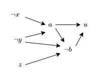
$\neg x$ and $\neg y$ mean $a$ has to be true by unit propagation on the first clause. $a$, $\neg y$ and $z$ mean $\neg b$ has to be true by unit propagation on the second clause. $a$ and $\neg b$ mean $u$ has to be true by unit propagation on the third clause.
A conflict literal $l$ is one for which both $l$ and $\neg l$ appear as nodes in the graph. This is a conflict because $l$ and $\neg l$ cannot be true at the same time. A conflict graph is a subgraph of the implication graph that contains
- exactly one conflict literal $l$
- only nodes that have a path to $l$ or $\neg l$
- incoming edges corresponding to one particular clause only
Consider an edge cut in the conflict graph that has all decision literals on one side of the cut $R$ and the conflict literals on the other side $C$ and all edges across the cut start in $R$ and end in $C$. A conflict clause is the clause obtained by considering all edges $l$ to $l'$ where $l \in R$ and $l' \in C$ and taking the disjunction of all literals $\neg l$. Different learning schemes are used to select which conflict clause to add. Any conflict clause can be inferred by the resolution rule from the existing clauses, so adding conflict clauses does not affect satisfiability.
Conflict-driven clause learning is an algorithm which uses conflicts in implication graphs to decide which clause to add to a formula.
- Select a variable and assign true or false
- Apply unit propagation
- Build the implication graph
- If there is any conflict, derive a corresponding conflict clause and add it to the formula, then non-chronologically backtrack to the decision level where the first assigned variable involved in the conflict was assigned
- Repeat step 1 until all variables are assigned
The solutions considered so far are complete. Monte Carlo methods are incomplete and based on stochastic local search. A simple example is starting with a random truth assignment to the variables. While there are unsatisfied clauses, pick any variable and flop a random literal in it, giving up after some number of trials. For a satisfiable 3-SAT formula with $n$ variables, this algorithm will succeed with probability $\Omega((3/4)^n/n)$ after at most $n$ rounds. If the algorithm is repeated $Kn(4/3)^n$ times for some large enough $K$ then it is almost certain to find a solution. This runs in $O((4/3)^n) \approx O(1.33^n)$ time, which is better than the naive $O(2^n)$ algorithm and the improved $O(1.913^n)$ algorithm but if the formula is not satisfiable, the algorithm will never prove this conclusively.
First-order logic
Every statement in propositional logic is either true or false, it has limited expressive power. First-order logic has the following features
- Propositional connectives and constants
- Quantifiers: $\forall$ and $\exists$
- Variables (not just true or false)
- Relation symbols: $>$, $=$, $p(x)$ where $x$ is prime
- Function symbols: $s(x)$ is the successor of $x$, $x+y$ is the sum of $x$ and $y$
- Constant symbols
For example, "every natural number has a successor" would be denoted $\forall x \exists y(y = s(x))$.
A first order language is determined by specifying
- A finite or countable set $\mathbf{R}$ of relation symbols or predicate symbols, each with some number of arguments
- A finite or countable set $\mathbf{F}$ of function symbols, each with some number of arguments
- A finite or countable set $\mathbf{C}$ of constant symbols
The language determined by $\mathbf{R}$, $\mathbf{F}$ and $\mathbf{C}$ is denoted $L(\mathbf{R}, \mathbf{F}, \mathbf{C})$.
The family of terms of $L(\mathbf{R}, \mathbf{F}, \mathbf{C})$ is the smallest set satisfying the following conditions
- Any variable is a term
- Any constant symbol (member of $\mathbf{C}$) is a term
- If $f$ is a function symbol (member of $\mathbf{F}$) with $n$ arguments and $t_1,...,t_n$ are terms then $f(t_1,...,t_n)$ is a term
An atomic formula of $L(\mathbf{R}, \mathbf{F}, \mathbf{C})$ is any string of the form $R(t_1, ..., t_n)$ where $R$ is a relation symbol (member of $\mathbf{R}$) with $n$ arguments and $t_1, ..., t_n$ are terms. $\top$ and $\bot$ are also taken to be atomic formulae.
The family of formulae of $L(\mathbf{R}, \mathbf{F}, \mathbf{C})$ is the smallest set satisfying the following conditions
- Any atomic formula is a formula of $L(\mathbf{R}, \mathbf{F}, \mathbf{C})$
- If $A$ is a formula, so is $\neg A$
- If $A$ and $B$ are formulae and $\circ$ is a binary connective then $(A \circ B)$ is also a formula
- If $A$ is a formula and $x$ is a variable then $\forall x A$ and $\exists xA$ are also formulae
The free-variable occurrences in a formula are defined as follows
- For an atomic formula, they are all the variable occurrences in that formula
- For $\neg A$ they are the free-variable occurrences in $A$
- For $(A \circ B)$, they are the free-variable occurrences in $A$ and $B$
- For $\forall x A$ or $\exists x A$, they are the free-variable occurrences of $A$ except for occurrences of $x$
If a variable occurrence is not free then it is bound. For example, in the formula $Q(x) \rightarrow \forall x R(x)$ the first occurrence of $x$ is free but the second is bound.
A sentence or closed formula of $L(\mathbf{R}, \mathbf{F}, \mathbf{C})$ is a formula with no free-variable occurrences.
First-order logic semantics
A model for the first-order language $L(\mathbf{R}, \mathbf{F}, \mathbf{C})$ is a pair $\mathbf{M} = (\mathbf{D}, \mathbf{I})$ where
- $\mathbf{D}$ is a non-empty set, called the domain of $\mathbf{M}$
- $\mathbf{I}$ is a mapping, called an interpretation, that associates
- to every constant symbol $c \in \mathbf{C}$, some member $c^\mathbf{I} \in \mathbf{D}$
- to every function symbol $f \in \mathbf{F}$ with $n$ arguments, some $n$-ary function $f^\mathbf{I}: \mathbf{D}^n \rightarrow \mathbf{D}$
- to every relation symbol $R \in \mathbf{R}$ with $n$ arguments, some $n$-ary relation $R^\mathbf{I} \subseteq \mathbf{D}^n$
An assignment in a model $\mathbf{M} = (\mathbf{D}, \mathbf{I})$ is a mapping $\mathbf{A}$ from the set of variables to the set $\mathbf{D}$. $x^\mathbf{A}$ denotes the image of $x$ under $\mathbf{A}$.
Let $\mathbf{M} = (\mathbf{D}, \mathbf{I})$ be a model for the language $L(\mathbf{R}, \mathbf{F}, \mathbf{C})$ and let $\mathbf{A}$ be an assignment in this model. Each term $t$ of the language is assigned a value $t^{\mathbf{I}, \mathbf{A}}$ as follows
- For a constant symbol, $c^{\mathbf{I}, \mathbf{A}} = c^\mathbf{I}$
- For a variable, $x^{\mathbf{I}, \mathbf{A}} = x^\mathbf{A}$
- For a function symbol $f$ with $n$ arguments, $(f(t_1,...,t_n))^{\mathbf{I}, \mathbf{A}} = f^\mathbf{I}(t_1^{\mathbf{I}, \mathbf{A}},...,t_n^{\mathbf{I}, \mathbf{A}})$
For example, consider the language $L(\emptyset, \{s, +\}, \{0\})$ and terms $t_1 = s(s(0) + s(x))$ and $t_2 = s(x+s(x+s(0)))$.
One model of this language is $\mathbf{D} = \mathbb{N}$, $0^\mathbf{I} = 0$, $s^\mathbf{I}$ is the successor function and $+^\mathbf{I}$ is the addition operation. If $\mathbf{A}$ is an assignment such that $x^\mathbf{A} = 3$ then $t_1^{\mathbf{I}, \mathbf{A}} = 6$ and $t_2^{\mathbf{I}, \mathbf{A}} = 9$.
Another model could be $\mathbf{D}$ is the set of all words over the alphabet $\{a,b\}$, $0^\mathbf{I} = a$, $s^\mathbf{I}$ appends $a$ to the end of a word and $+^\mathbf{I}$ is concatenation. If $A$ is an assignment such that $x^\mathbf{A} = aba$ then $t_1^{\mathbf{I}, \mathbf{A}} = aaabaaa$ and $t_2^{\mathbf{I}, \mathbf{A}} = abaabaaaaa$. This shows how the same language can have different semantics under different models and assignments.
Let $\mathbf{M} = (\mathbf{D}, \mathbf{I})$ be a model for the language $L(\mathbf{R}, \mathbf{F}, \mathbf{C})$ and let $\mathbf{A}$ be an assignment in this model. Each formula $\phi$ of $L(\mathbf{R}, \mathbf{F}, \mathbf{C})$ has a truth value $\phi^{\mathbf{I}, \mathbf{A}}$ as follows
- $R(t_1, ..., t_n)^{\mathbf{I}, \mathbf{A}} = \text{true}$ if and only if $(t_1^{\mathbf{I}, \mathbf{A}},...,t_n^{\mathbf{I}, \mathbf{A}}) \in R^\mathbf{I}$
- $\top^{\mathbf{I}, \mathbf{A}} = \text{true}$
- $\bot^{\mathbf{I}, \mathbf{A}} = \text{false}$
- $(\neg X)^{\mathbf{I}, \mathbf{A}} = \neg(X^{\mathbf{I}, \mathbf{A}})$
- $(X \circ Y)^{\mathbf{I}, \mathbf{A}} = X^{\mathbf{I}, \mathbf{A}} \circ Y^{\mathbf{I}, \mathbf{A}}$
- $(\forall x \phi)^{\mathbf{I}, \mathbf{A}} = \text{true}$ if and only if $\phi^{\mathbf{I}, \mathbf{A'}} = \text{true}$ for every assignment $\mathbf{A'}$ that differs from $\mathbf{A}$ by the value assigned to $x$
- $(\exists x \phi)^{\mathbf{I}, \mathbf{A}} = \text{true}$ if and only if $\phi^{\mathbf{I}, \mathbf{A'}} = \text{true}$ for some assignment $\mathbf{A'}$ that differs from $\mathbf{A}$ by the value assigned to $x$
A formula $\phi$ of $L(\mathbf{R}, \mathbf{F}, \mathbf{C})$ is true in the model $\mathbf{M} = (\mathbf{D}, \mathbf{I})$ if $\phi^{\mathbf{I}, \mathbf{A}}$ is true for all assignments $\mathbf{A}$.
A formula is valid if it is true in all models for the language.
A set of formulae $S$ is satisfiable in $\mathbf{M} = (\mathbf{D}, \mathbf{I})$ if there is an assignment $\mathbf{A}$ such that $\phi^{\mathbf{I}, \mathbf{A}}$ is true for all $\phi \in S$.
Formal theorem proving is usually concerned with establishing that a formula is valid. Arbitrary formulae can be turned into sentences by universally quantifying free variables. A sentence $X$ is a logical consequence of a set $S$ of sentences, denoted $S \vDash X$ if $X$ is true in every model in which all the members of $S$ are true.
First-order proof systems
The propositional proof procedures can be extended to prove first-order logic. As well as $\alpha$ and $\beta$ formulae, first-order proof systems use $\gamma$ and $\delta$ formulae as well. $\gamma$ formulae are universally quantified and $\delta$ are existentially quantified.
Universal
| $\gamma$ | $\gamma(t)$ |
|---|---|
| $\forall x \phi$ | $\phi\{x/t\}$ |
| $\neg\exists x \phi$ | $\neg\phi\{x/t\}$ |
Existential
| $\delta$ | $\delta(t)$ |
|---|---|
| $\exists x \phi$ | $\phi\{x/t\}$ |
| $\neg\forall x \phi$ | $\neg\phi\{x/t\}$ |
where $\phi\{x/t\}$ denotes the formula obtained from $\phi$ by replacing the free variable occurrences of the variable $x$ with the term $t$.
Given $L(\mathbf{R}, \mathbf{F}, \mathbf{C})$, let $\mathbf{par}$ be a countable set of constant symbols that are disjoint from $\mathbf{C}$. The elements of $\mathbf{par}$ are called parameters and $L^\mathbf{par}$ is a shorthand for $L(\mathbf{R}, \mathbf{F}, \mathbf{C} \cup \mathbf{par})$.
First-order tableau
For tableau proof, $\gamma$-formulae add new node with $\gamma(t)$ where $t$ is any closed (no variables) term of $L^\mathbf{par}$ and $\delta$-formulae add a new node with $\delta(p)$ where $p$ is a new parameter that has not yet been used in the proof tree. Proofs will be of sentences of $L$, but they use sentences of $L^\mathbf{par}$.
An example tableau proof for $\forall x(P(x) \vee Q(x)) \rightarrow (\exists x P(x) \vee \forall x Q(x))$:
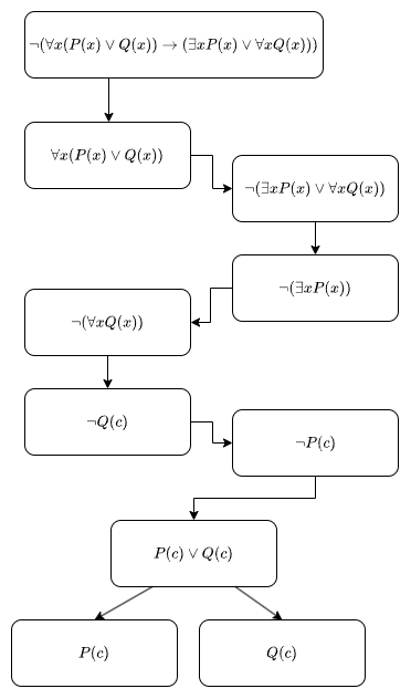
The first four children are derived from alpha expansion. The $\delta$ rule is applied to $\neg(\forall x Q(x))$ with parameter $c$ (this does not have special meaning, it is just a new parameter, it could be called $d$ instead) to give $\neg Q(c)$. The $\gamma$ rule is applied to $\neg(\exists x P(x))$ to give $\neg P(c)$, where $c$ is used as the replacement term. A different term could be substituted but this would not lead to a contradiction. Finally, $\forall x(P(x) \vee Q(x))$ becomes $P(c) \vee Q(c)$ by the $\gamma$ rule. This is then beta-expanded to give a contradiction on both branches. This is a closed tableau, so the original formula is valid.
As before, tableau rules are non-deterministic, but it is usually advantageous to do delta rules before gamma rules as the gamma rules can use the new parameters, making a contradiction easier. It is not possible to strictly apply the $\gamma$ rule, so heuristics are needed instead.
First-order resolution
Resolution works similarly to tableau. $\gamma$ formula are replaced with $\gamma(t)$ and $\delta$ with $\delta(p)$.
The resolution proof for $\forall x(P(x) \vee Q(x)) \rightarrow (\exists x P(x) \vee \forall x Q(x))$ (same as the tableau example) is as follows:
- Take negation: $\left[\neg(\forall x(P(x) \vee Q(x)) \rightarrow (\exists x P(x) \vee \forall x Q(x)))\right]$
- $\alpha$-expansion on 1: $\left[\forall x(P(x) \vee Q(x))\right]$ and $\left[\neg(\exists x P(x) \vee \forall x Q(x))\right]$
- $\alpha$-expansion on 2b: $\left[\neg\exists x P(x)\right]$ and $\left[\neg\forall x Q(x)\right]$
- $\delta$-expansion on 3b: $\left[\neg Q(c)\right]$
- $\gamma$-expansion on 3a: $\left[\neg P(c)\right]$
- $\gamma$-expansion on 2a: $\left[P(c) \vee Q(c)\right]$
- $\beta$-expansion on 6: $\left[P(c), Q(c)\right]$
- Resolution rule on $P(c)$ for 5 and 7: $\left[Q(c)\right]$
- Resolution rule on $Q(c)$ for 4 and 8: $\left[\;\right]$
First-order tableau and resolution are sound and complete. I will not elaborate.
First-order natural deduction
$\gamma$ and $\delta$ formulae can be replaced as with resolution for natural deduction. The natural deduction proof of $\forall x(P(x) \rightarrow Q(x)) \rightarrow (\forall xP(x) \rightarrow \forall x Q(x))$ is as follows
- ┏ $\forall x(P(x) \rightarrow Q(x))$ (assumption)
- ┃┏ $\forall x(P(x)$ (ass.)
- ┃┃┏ $\neg(\forall x Q(x))$ (ass.)
- ┃┃┃ $\neg Q(p)$ ($\delta$-elimination on 3)
- ┃┃┃ $P(p)$ ($\gamma$-elimination on 2)
- ┃┃┃ $P(p) \rightarrow Q(p)$ ($\gamma$-elimination on 1)
- ┃┃┃ $Q(p)$ (modus ponens on 5 and 6)
- ┃┃┗ $\bot$ (negation on 4 and 7)
- ┃┗ $\forall x Q(x)$ (contradiction)
- ┗ $\forall xP(x) \rightarrow \forall x Q(x)$ (impl.)
- $\forall x(P(x) \rightarrow Q(x)) \rightarrow (\forall xP(x) \rightarrow \forall x Q(x))$ (impl.)
First-order natural deduction is sound and complete. Proof is left as an exercise to the reader.
Program verification
Program verification is used to determine if a property holds for a program, denoted $P \vdash \phi$ where $P$ is the program and $\phi$ is the property. An example is x=0; i=1; while(i<=n) { x=x+arr[i]; i=i+1 } $\vdash x = \sum_{i=1}^n \text{arr}[i]$, which verifies that the program finds the sum of the array.
Program verification uses a simple programming language. It consists of three syntactic domains, integer expressions E, boolean expressions B and commands C. The commands include
- assignment,
x = E - composition,
C1; C2 - conditional,
if B then {C1} else {C2} - loops,
while B {C}
The postcondition is the property that must hold when the execution of a program terminates. It is a first-order logic formula referring to program variables which express the conditions formally.
The precondition is the property that program variables must satisfy before the program starts and is also a first-order logic formula. The precondition can also be $\top$, meaning there are no preconditions.
A Hoare triple consists of the precondition, program and postcondition, denoted (|Pre|) Prog (|Post|). This is a logical statement which may be true or false for different values of Pre, Prog and Post.
Examples
- (|$y=1$|) $x = y+1$ (|$x=2$|) is true
- (|$y=1$|) $x = y+1$ (|$x>y$|) is true
- (|$y=1$|) $x = y+1$ (|$x=1$|) is false
- (|$y=1$|) $x = y+1$ (|$z=0$|) is false
From the given precondition we must guarantee that the postcondition is always reached.
Weakest precondition
The weakest precondition (WP) for a program to establish a postcondition is a precondition guaranteeing that the postcondition holds and that it is implied by any other possible precondition, denoted wp(P, Post). It is the minimum requirement for P to successfully reach the postcondition.
Weakest preconditions can be computed formally for each language construct. For assignments, the WP will be the postcondition replaced with the new value. For example, (|?|) x=x+1 (|x>3|) would have WP x+1>3 which is x > 2. Formally, wp(x=E, Post) = Post[x/E] where Post[x/E] is Post with x replaced with E.
Examples
- wp(
x=y,x=6) isx=y[x/y] which isy=6 - wp(
x=1,x>0) isx>0[x/1] which is1 > 0which is $\top$ - wp(
x=0,x>0) isx>0[x/0] which is0 > 0which is $\bot$ - wp(
z=x, $(z \geq x \wedge z \geq y)$) is $(z \geq x \wedge z \geq y)$[z/x] which is $(x \geq x \wedge x \geq y)$ which is $\top \wedge x \geq y$ which is $x \geq y$ - wp(
i=i+1,j=6) isj=6
The WP for composite assignments is wp(P; Q, Post) = wp(P, wp(Q, Post)). For example, wp(x=y+2; y=2*x, x+y>20) is wp(x=y+2, 3*x>20) which is 3*(y+2) > 20 which is 3y > 14.
The WP for conditionals, wp(if B then {C1} else {C2}, Post), is (B $\rightarrow$ wp(C1, Post)) $\wedge$ (¬B $\rightarrow$ wp(C2, Post)) or equivalently (B $\wedge$ wp(C1, Post)) $\vee$ (¬B $\wedge$ wp(C2, Post)).
For example, wp(if x>0 then {y=x} else {y=-x}, $y = \left|x\right|$) gives $(x>0 \rightarrow x = \left|x\right|) \wedge (\neg(x>0) \rightarrow -x = \left|x\right|)$ which is $\top$.
Hoare logic
Any program is a sequence of instructions, Prog = C1; C2; ...; Cn. A proof for Prog shows the preconditions for each command which can then be composed to verify the whole program.
The assignment rule states that (|Post[x/E]|) x = E (|Post|) is a valid Hoare triple and can be introduced wherever an assignment occurs.
The implied rule states that if Pre $\rightarrow$ P then (|P|) Prog (|Post|) can be replaced with (|Pre|) Prog (|Post|). If Q $\rightarrow$ Post then (|Pre|) Prog (|Q|) can be replaced with (|Pre|) Prog (|Post|). This corresponds to strengthening the precondition or weakening the postcondition.
The composition rule states that if (|Pre|) Prog1 (|Mid|) and (|Mid|) Prog2 (|Post|) are valid then (|Pre|) Prog1; Prog2 (|Post|) is valid.
A proof for (|$y = 10$|) x = y-2 (|$x>0$|) would first use the assignment rule to derive (|$y > -2$|) as a precondition which is then used to derive (|$y = 10$|) by the implied rule. Similar to natural deduction proofs, these proofs are built upwards and then read downwards.
The conditional rule states that if (|Pre $\wedge$ B|) C1 (|Post|) and (|Pre $\wedge$ ¬B|) C2 (|Post|) are valid then (|Pre|) if B {C1} else {C2} (|Post|) is valid.
Consider (|$\top$|) if (x<y) then {z=x} else {z=y} (|$z \leq x \wedge z \leq y$|). Applying assignment gives $x \leq x \wedge x \leq y$ for the first branch and $y \leq x \wedge y \leq y$ for the second, which can be simplified to $x \leq y$ and $y \leq x$ respectively. These can be changed to $x < y$ and $\neg(x < y)$ respectively by the implied rule. Given these, the conditional rule can be applied to give $\top$. The proof is shown below.
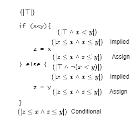
The loop rule states that if (|B $\wedge$ L|) C (|L|) is valid then (|L|) while B {C} (|¬B $\wedge$ L|) is valid where L is the loop invariant. The loop invariant holds before and after each iteration.
CS263 - Cyber Security
Cyber security is the application of technologies, processes and controls to protect systems, networks, programs, devices and data from cyber attacks.
Brief history
- 1940s - First computer
- 1950s - Telephone hacking
- 1971 - Creeper for ARPANET, the first worm
- 1972 - Reaper, which removed Creeper, the first antivirus
- 1983 - US Department of Defence published Trusted Computer System Evaluation Criteria
- 1987 - First commercial antiviruses
- 1988 - Morris worm, first charge under 1986 Computer Fraud and Abuse Act
- 1991 - First polymorphic virus
- 1994 - SSL protocol developed
- 1999 - Melissa macro virus
- 2010 - Stuxnet worm
- 2017 - Wannacry ransomware
- 2021 - Log4Shell
Cybersecurity threats
- Destruction of data
- Unauthorised modification of data
- Theft of data
- Disclosure of data
- Interruption of services
Examples of exploits:
- Buffer overflow - A program attempts to put more data in a buffer than it can hold. Writing outside the bounds of a block of allocated memory can allow for the execution of malicious code.
- Man in the middle attack - An attacker intercepts and relays messages between two parties
- Denial of service attack - Attacker prevents authorised users from accessing a service
- Zero day exploit - A vulnerability discovered by an attacker before the vendor is aware of it
- Backdoor - A method of bypassing normal authentication to gain unauthorised access to a system
- Trojan - A program with a hidden malicious purpose
Kali Linux
Kali Linux is a Debian-based Linux distribution designed for digital forensics and penetration testing. It includes lots of tools including
- nmap - Port scanning
- John the Ripper - Password cracking
- Wireshark - Packet sniffing
- Burpsuite - Web application testing
- Autopsy - Forensic analysis
- GPG - Signatures and encryption
- Steghide - Steganography (hiding data in an image)
- Metasploit Framework - Penetration testing
Penetration testing
Penetration testing consists of 3 main stages: preparation, testing and reporting.
Preparation can include
- Interviewing the client to assess their concerns
- Determining the scope of testing
- Signing a penetration testing agreement
- Define the rules of engagement
When testing, it is important to only carry out the testing requested and consider relevant laws of all countries the testing takes place in.
Once testing has been completed, the findings can be compiled into a report. This explains to the client the vulnerabilities found, their severity and what can be done to mitigate them.
Reconnaissance
The aim of reconnaissance is to determine a list of targets to be scanned, assessed and exploited.
Open source intelligence (OSINT) is intelligence derived from publicly available sources. These sources may include websites, social media, job listings, arrest records, DNS records, archives and image metadata.
Scanning
Scanning is used to discover a system's vulnerabilities. Host discovery can be used for find hosts which are alive. Port scanning can be used to find vulnerable open ports. Tools like netstat, nmap, tcpdump, traceroute and wireshark can be used to analyse networks and read packets.
Exploitation
An exploit takes advantage of a vulnerability to perform an attack. It is important to not breach the rules of engagement when exploiting a system.
A common exploit payload is a shell. There are type types - bind and reverse shells. Bind shells open a port which listens for connections on the target whereas a reverse shell connects the target back to the attacker. A bind shell may be blocked by a firewall so reverse shells are usually more successful.
Web shells are malicious scripts installed onto a web server. They act as a backdoor and allow the attacker access to the web server. This attack can be prevented by using file integrity monitoring and suitable permission settings.
Web application testing
The OWASP testing guide describes four testing techniques
- Manual inspections and reviews - Human reviews which test the security implications of people, policies and procedures
- Threat modelling - Risk assessment for applications
- Source code review - Manually checking source code for vulnerabilities
- Penetration testing
Several tools exist for testing web application security. Examples include
- w3af - Attack and audit framework
- sqlmap - SQL injection detector
- Hydra - login cracker
- Nessus - vulnerability scanner
- ZAP - man in the middle proxy, intercepts communications
- Burp suite - Contains several tools for web application testing
Fuzzing is a software testing technique which random, invalid or unexpected data to find vulnerabilities.
Bug bounty programs incentivise the finding and disclosure of bugs in a program by offering a financial reward.
Web application attacks can be mitigated by performing vulnerability scanning, using a web application firewall (WAF) and secure development testing.
There are many types of web application attack, including
- Cross site scripting (XSS)
- Path traversal
- Clickjacking
- Cross site request forgery (CSRF)
- Reflected DOM injection
- SQL injection
A Same Origin policy only allows Javascript from the same host to run on a website. Cross site scripting can bypass this by manipulating a vulnerability in a website and returning malicious code to a user. There are three types of XSS attack
- Reflected XSS - from the current HTTP request
- Stored XSS - from the website's database
- DOM-based XSS - from a vulnerability in client-side code
Program security
Some common vulnerabilities include
- Stack overflow - memory used by a recursive function exceed stack capacity
- Buffer overflow - Accessing memory outside of allocated buffer
- Access after deallocation
- Uninitialised variables
- Time of check to time of use flaws
- Side channel attacks - uses timing or processor utilisation to gather information
Application vulnerabilities can be found using three methods
- Static code analysis - Checks source code for flaws without executing it
- Reverse engineering - analyse binary/assembly
- Fuzzing - Fuzz inputs until something happens
GRC
GRC stands for Governance, Risk management and Compliance. It is a way to align cyber security with business goals while managing risk and complying with regulations.
Governance is the set of policies that a company uses to achieve its business goals. It defines the responsibilities of key stakeholders. Risk management considers potential problems and how they can be managed and compliance ensures a business complies with any laws and regulations necessary. Cyber security can be taken into consideration for all of these principles.
Hashing
A hash function maps data of any size to a fixed size output. Hash functions are one-way, meaning they are computationally hard to reverse.
Message Authentication Codes (MAC) are keyed hash functions. It uses a key to hash data. The same key can be used by the recipient to check the hash matches and authenticate the sender.
The birthday paradox states that only 23 people are needed for the probability that two of them share a birthday to be greater than 50%. The birthday attack on a hash function exploits this probability. A good hash function should require an attacker to compute as many hashes as possible before finding a match.
Hashing can be used to ensure data integrity and to provide digital signatures.
Hashing is used to store passwords securely but common passwords will have the same hash, making them easy to crack. A salt is random data appended to a password which prevents this. In addition to this, a salted hash can then be peppered with a secret key stored separately to the passwords.
Hashing is also used for blockchain transactions.
Contingency planning
Contingency planning is how an organisation handles and unexpected event or incident. It aims to resume normal operation with minimal cost and disruption after an adverse event.
There are 4 types of contingency planning
- Incident response - planning and preparation for detecting, reacting to and recovering from an incident
- Disaster recovery - Recover assets after a disaster
- Business continuity - Ensure business operations can continue after a disaster with as little downtime as possible
- Crisis management - Overall management of emergencies
Contingency planning includes making backups and having backup servers.
Threat modelling
Threat modelling identifies, communicates and prioritises threats and proposes mitigations.
One threat model is STRIDE. Each threat and the security property it threatens are as follows
- Spoofing - authentication
- Tampering - integrity
- Repudiation - non-repudiation
- Information disclosure - confidentiality
- Denial of service - availability
- Elevation of privilege - authorisation
DREAD uses a formula to evaluate vulnerabilities. Risk value = (Damage + Affected users) x (Reproducibility + Exploitability + Discoverability)
Open Authentication (OAuth) allows third-party application to access a user's account from another service without giving the third-party any credentials. Third-parties are granted access tokens from the OAuth service.
Various cyber security tools
- CashCat can be used to deliver a ransomware attack
- foremost can be used to retrieve deleted files
- Ettercap can be used to perform an ARP spoofing attack
- Maltego is an information gathering tool
Various cyber security topics
Social engineering uses psychological manipulation to deceive victims into making a mistake. It relies on human error rather than vulnerabilities in software.
Physical security protects buildings and equipment.
Digital forensics is a branch of forensic science which focusses on recovery and investigation of devices used for cybercrime. Digital forensics is the process of identifying, preserving, analysing and documenting digital evidence.
CS313 - Mobile Robotics
A robot is
- An artificial device that can sense its environment and act purposefully in it
- An embodied artificial intelligence
- A machine that can autonomously carry out useful work
Some advantages of using robots include
- Increased productivity, efficiency, quality and consistency
- Can repeat the same process continuously
- Very accurate
- Can work in environments which are not safe for humans
- Don't have the same physical or environmental needs as humans
- Can have sensors and actuators which exceed human capability
Some disadvantages include
- Robots replacing human jobs
- Limited by their programming
- Can be less dexterous than humans
- Limitations of robot vision
- High upfront cost
All real robots interact with humans to some extent. This ranges from autonomous (least human interaction) to commanded to remote controlled (most human interaction).
There are several ways in which a robot can be made to behave more intelligently
- Pre-program a larger number of behaviours
- Design the robot so that it explicitly represents the uncertainty in the environment
- Design the robot so it can learn and develop its own intelligence
A mobile robot is one which is capable of moving around its environment and performing certain tasks. The ability to move extends the workspace of a mobile robot, making it more useful.
Sensing
Robots have to be able to accommodate the uncertainty that exists in the physical world. Sensors are limited in what they can perceive and motors can also be unpredictable. Robots have to work in real time so have to make use of abstractions and approximations to ensure timely response at the cost of accuracy. This uncertainty can be represented using probabilistic methods.
Probabilistic methods represent information using probability distributions. These methods scale much better to complex and unstructured environments but have higher computational complexity, hence the need to approximate.
The sensing process consists of
- transduction - converts physical or chemical quantity into an electrical signal
- signal conditioning - makes signal linear and proportional to the quantity being measured
- data reduction and analysis - data used to generate a model of the world
- perception - models analysed to infer about the state of the world
Robot sensors can be classified based on their characteristics, such as what they measure, the technology used or the energy used.
One classification is whether the sensor is measuring something internal (proprioceptive (PC), such as power consumption) or external (exteroceptive (EC), such as light intensity) to the robot. Another is whether the sensor is passive (just listening) or active (emitting signals). An active sensor changes the environment and could cause interference to itself or other nearby robots.
Another way sensors can be categorised is by their performance, including
- bandwidth or frequency
- response time
- accuracy - difference between true value and measured value
- precision - repeatability
- resolution
- linearity
- sensitivity
- measurement range
- error rate
- robustness
- power, weight, size
- cost
Commonly used sensors include
- wheel/motor sensors
- heading sensors
- accelerometers
- inertial measurement units
- light and temperature sensors
- touch sensors
- proximity sensors
- range sensors
- beacons
- vision sensors
Wheel/motor encoders measure the position or speed of wheels or steering. These movements can be integrated to get an estimate of position, known as odometry or dead reckoning. They use light to produce pulses which can be used to detect revolutions. These sensors are simple and widely available but need line of sight.
Heading sensors determine the robot's orientation and inclination with respect to a given reference. Heading sensors can be proprioceptive (gyroscope, accelerometer) or exteroceptive (compass, inclinometer). Allows the robot to integrate the movement to a position estimate.
Gyroscopes provide an absolute measure of the heading of a mobile system. They are useful for stabilisation or measuring heading or tilt. Mechanical gyroscopes use a spinning rotor and optical gyroscopes use laser beams.
An inclinometer measures an incline. This can be done with mercury switches or electrolyte sensors. A mercury switch is a glass bulb with a drop of mercury and two contacts. If the robot is on an incline the mercury will connect the contacts, providing a binary signal. Electrolyte signals produce a range of signals depending of the degree of tilt.
Accelerometers measure acceleration. They work on the principle of a mass on a string. When the robot accelerates the string is stretched or compressed creating a force which can be detected. Accelerometers measure acceleration along a single axis. These can be measured using resistive, capacitive or inductive techniques.
Micro-electromechanical system (MEMS) accelerometers use a fixed body with a proof mass and finger electrodes. When subjected to acceleration the proof mass resists motion causing the electrodes to touch it can carry a signal. These sensors are cheap to produce but have limited depth of field and the signal needs to be integrated.
Accelerometers, gyroscopes and heading sensors can be combined with an Inertial Measurement Unit (IMU). The IMU uses signals from the sensors to estimate the relative position, orientation, velocity and acceleration of a moving vehicle with respect to an inertial frame. It needs to know the gravity vector and initial velocity. IMUs are extremely sensitive to measurement errors and drift after being used for a long time.
Light sensors detect light and create a voltage difference. The two main types are photoresistor and photovoltaic cells. Photoresistors a resistors whose resistance varies with light intensity. Photovoltaic cells convert solar energy into electrical energy.
Temperature sensors use thermistors to measure temperature change using resistance like a photoresistor.
Touch sensors are broadly classified into contact sensors and tactile sensors. Contact sensors just measure contact with an object whereas tactile sensors measure roughness of an object's surface.
A basic contact sensor is a switch which generates a binary signal. These are simple and cheap but not passive and provide limited information.
Tactile sensors use piezoelectric materials which can convert mechanical energy to electrical energy. This allows them to determine the hardness of a surface.
Passive InfraRed (PIR) sensors detect IR. It uses two IR detectors and when one detects IR it causes a differential change between the two sensors. These sensors are simple and cheap but only provide binary detectors and are very noisy.
Range sensors measure the distance from the robot to an object in the environment. This can be used for obstacle avoidance or constructing maps. Range can be measured using time of flight, phase shift or triangulation.
Time of flight ranging makes uses of the propagation of the speed of sound, light or an electromagnetic wave to calculate range. SONAR uses sound and LIDAR uses light.
Phase shift measurement measures phase shift between two beams, one which reflects off a splitter an object and the other that reflects off the splitter only. Phase shift is constrained to a specific range of 0 to 360 degrees. If the shift exceeds this range then it wraps around making range estimates ambiguous.
Triangulation ranging detects range from two points at a known distance from each other. These distances and angles can be used to calculate the distance to an object.
Active IR sensors are devices that use IR light to detect objects. Unlike passive sensors, active sensors emit their own IR and measure the reflected signal but aren't very accurate.
SONAR uses sound ultrasonic sound to determine range. Sound is emitted and the reflection is received. They are quite simple and widely used but are vulnerable to interference and have limited range and bandwidth.
RADAR works like SONAR but with high frequency radio waves. This is cheap and accurate with longer range but needs beam forming, signal processing and is vulnerable to interference.
LIDAR uses lasers to detect range. This is fast and accurate but has limited range, uses a lot of power, is expensive and vulnerable to interference from other sensors and transparent or reflective surfaces.
Beacons can be used to localise a robot in an external reference frame. Active or passive beacons with known locations can be used for robot localisation. Several beacons can be used with trilateration to identify a robot's position. GPS uses satellite beacons which can be picked up by a receiver which uses trilateration to calculate its position. GPS uses 4 satellites to calculate time correction as well as position because time errors are critical. Differential GPS uses land-based receivers which exactly known locations which receive signals, compute correction and rebroadcast the signal. This improves the accuracy and availability of GPS.
Vision
The two current technologies for vision sensors are CCD and CMOS cameras. The CCD chip is an array of light-sensitive pixels which capture and count photons. The pixel charges are then read on each row.
The CMOS chip consists of an array of pixels with several transistors for each pixel. Like CCD the pixels collect photons but each pixel can count its own signal.
Basic light measuring is colourless. There are two approaches to sensing colour. A three chip colour camera splits the incoming light into three copies which are passed to a red, green and blue sensor. This is expensive. An RGB filter is more commonly used and cheaper. It groups pixels and applies a colour filter so that each pixel only receives light of one colour. Usually 2 pixels measure green and 1 measures red and blue each. This is because luminance values are mostly determined by green light and luminance is more important than chrominance for human vision.
Both colour sensors suffer from the fact that photodiodes are much more sensitive to near infrared light so capture blue worse than red and green.
There are several colour spaces
- RGB (Red, Green, Blue)
- CMYK (Cyan, Magenta, Yellow, Black)
- HSV (Hue, Saturation, Value)
The more pixels captured by a chip in a given area the higher the resolution. Even inexpensive cameras can capture millions of pixels in a single image. The problem with high resolution is the large amount of memory needed to store them and the computing power required to analyse them. The resolution of an image can be reduced with pixel deletion or colour reduction.
A pinhole camera works by using a small hole called an aperture which only lets a little light in. This produces a dark image. Instead, a lens is used to focus light to a focal point which keeps focus while keeping the image brighter.
The thin lens model is a basic lens model. The relationship between the distance to an object, $u$, and the distance behind the lens at which the focused image is formed, $v$, can be expressed as $$ \frac{1}{f} = \frac{1}{u} + \frac{1}{v} $$ where $f$ is the focal length. Any object point satisfying this equation is in focus. This formula can also be used to estimate the distance to an object.
Perspective projection is a technique used to represent a three dimensional scene onto a two dimensional surface. The 3d scene point $P = (x, y, z)$ can be expressed as a 2d image point $\left(\frac{f}{z}x, \frac{f}{z}y\right)$ where $f$ is the focal length. This mapping is non-linear, so projective geometry has an extra dimension, $w$. This is a scaling transformation for the 3d coordinate. Coordinates in projective space are called homogeneous coordinates. The projection equation written using homogeneous coordinates is $$ \begin{bmatrix} \lambda u\\\lambda v\\\lambda\end{bmatrix} = \begin{bmatrix} fx \\ fy \\ z\end{bmatrix} = \begin{bmatrix} f & 0 & 0 & 0\\ 0 & f & 0 & 0\\ 0 & 0 & 1 & 0\end{bmatrix} \begin{bmatrix}x\\y\\z\\1\end{bmatrix} $$ where $u$ and $v$ are the image coordinates, $\lambda$ is the depth and $f$ is the focal length.
A realistic camera model that describes the transformation from 3D coordinates to pixel coordinates must also take into account the pixelisation of the sensor and rigid body transformation between the camera and the scene. In general, the world and the camera do not have the same reference frame, so another transformation is introduced to give the camera matrix: $$ \begin{bmatrix} \lambda u\\\lambda v\\\lambda\end{bmatrix} = \begin{bmatrix} fk_u & 0 & u_0 & 0\\ 0 & fk_v & v_0 & 0\\ 0 & 0 & 1 & 0\end{bmatrix}\begin{bmatrix} r_{11} & r_{12} & r_{13} & t_1\\ r_{21} & r_{22} & r_{23} & t_2 \\ r_{31} & r_{32} & r_{33} & t_3\\0 & 0 & 0 & 1\end{bmatrix} \begin{bmatrix}x\\y\\z\\1\end{bmatrix} $$ where $u_0, v_0$ are the coordinates of the principal point (corrects the optical center of the image), $k_u$ and $k_v$ are horizontal and vertical scale factors (corrects pixel size), $r_{11}\dots r_{33}$ rotate the image and $t_1 \dots t_3$ translate the image to make it match the world reference frame. These values are usually determined through calibration.
Depth of field is the distance between the closest and farthest objects in a photo that appears acceptably sharp. The size of the aperture controls the amount of light entering the lens. A smaller aperture increases the range in which the object is approximately in focus.
Field of view (FOV) is an angular measure of the portion of 3D space that can be captured by a camera. It is typically measured in degrees. Wider FOV captures more of the scene whereas a narrower field focuses on a smaller portion, making objects appear larger and more magnified. The FOV is influenced by the focal length of the lens. Shorter focal lengths generally result in wider FOVs whereas longer focal lengths result in narrower FOVs.
Structure from stereo is one method of recovering depth information. It uses two images from two cameras at a known relative position to each other. The $z$ coordinate can be estimated as $b\frac{f}{u_l-u_r}$ where $b$ is the baseline which is the distance between the cameras and $u_l$ and $u_r$ are the difference in the image coordinates between the cameras, called the disparity.
Structure from motion is another method in which the relation position of the cameras is not known. Images are taken at different positions or times. Both structure and motion must be estimated simultaneously. This can produce results comparable to laser range finders but requires expensive computation.
Some methods of image processing include
- Pixel processing - transform pixel by pixel
- Convolution - apply a mask/filter to the image
- Smoothing filter - blurring and noise reduction, Gaussian filter for example
- Line detection - detects lines
- Median filter - removes salt and pepper noise
Edges are significant local changes to the intensity of an image. They typically occur on the boundary between two different regions in an image. Edges are extracted from greyscale images and can be used to produce a line drawing of a scene.
Edges characterise discontinuities in an image. Edges can be modelled according to their intensity profiles, either step, roof, ramp or spike. Points which lie on an edge can be detected by detecting the local maxima or minima of the first derivative and detecting the zero-crossing of the second derivative.
One method of edge detection is using the image gradient. Partial derivatives of a 2D continuous function represent the amount of change along each direction. These derivatives can be used to calculate magnitude and orientation of edges. Because images are discrete, a convolution filter can be used instead. Two examples of gradient filters are Prewitt and Sobel filters. There are filters for detecting horizontal, vertical and diagonal lines.
Another method is using the Laplacian of an image. It considers the first and second derivatives to detect edges. It does not provide orientation.
The Canny edge detector algorithm:
- Smooth the image with the Gaussian filter
- Compute the gradient
- Find the gradient magnitude and orientation
- Apply non-maximum suppression to the thin edges
- Track edges by hysteresis
Corner detection can be used for feature detection. Corner detection can either be based on image brightness or boundary extraction.
The Harris corner detector can be used to detect corners
- Compute the image gradients using a derivative filter (such as the Sobel filter) in both the $x$ and $y$ directions
- Use the gradients to create a structure tensor for each pixel in the image. The structure tensor is a 2x2 matrix that summarises the local intensity variations in the neighbourhood of a pixel
- Use the structure tensor to compute a scalar value for each pixel, known as the corner response function
- Apply non-maximum suppression to the corner response map to identify the local maxima. This helps filter out multiple responses around a single corner
- Apply a threshold to the corner response values to identify significant corners. Pixels with corner response values above the threshold are considered corners
Harris corner detection is invariant to rotation and partially invariant to intensity change but is not invariant to image scale.
Scale Invariant Feature Transform (SIFT) transforms image data into scale-invariant coordinates. It is robust to affine distortion, change in 3D viewpoint, noise and changes in illumination. SIFT works as follows
- Find extrema in scale space
- Find the location of key points
- Assign an orientation to each keypoint
- Describe the keypoint using the SIFT descriptor
State estimation
The robot's initial belief about its position in the world can be modelled as a uniform probability density function (PDF). As the robot senses things, the PDF can be updated to reflect this new knowledge. When the robot moves the belief PDF is shifted in the direction of motion and peaks are spread. When the robot takes another sensor measurement, the belief PDF can be updated to give a higher probability of the robot's position.
Bayes theorem is $$ P(x|y) = \frac{P(y|x)P(x)}{P(y)} $$
The posterior state estimation given sensor measurements $z$ and control inputs $u$ is given by $\operatorname{Bel}(x_t) = p(x_t | u_1, z_1, \dots u_t, z_t)$.
The recursive Bayes filter can be derived as follows: $$ \begin{aligned} \operatorname{Bel}(x) &= p(x_t | u_1, z_1, \dots, u_t, z_t)\\ &= \eta p(z_t | x_t, u_1, z_1, \dots, u_t)p(x_t | u_1, z_1, \dots, u_t) & \text{Bayes rule}\\ &= \eta p(z_t | x_t) p(x_t | u_1, z_1, \dots, u_t) & \text{Sensor independence}\\ &= \eta p(z_t | x_t) \int p(x_t | u_1, z_1, \dots, u_t, x_{t-1}) p(x_{t-1} | u_1, z_1, \dots, u_{t-1}, z_{t-1}) dx_{t-1} & \text{Law of total probability}\\ &= \eta p(z_t | x_t) \int p(x_t | u_t, x_{t-1}) \operatorname{Bel}(x_{t-1}) dx_{t-1} & \text{Markov assumption} \end{aligned} $$ where $\eta$ is a normalising constant.
To implement this, the observation and motion models need to be specified based on the dynamics of the system and the belief representation needs to be determined.
A discrete Bayes filter can be used for problems with finite state spaces. The integral can be replaced with a summation. In practice, the probabilities can be represented by matrices and the belief propagation can be done with matrix multiplication.
The filter can be expressed using matrix multiplication as follows $$ (\bm{\hat{f}}_ {0:t})^T = c^{-1}\bm{O}_ t(\bm{T})^T(\bm{\hat{f}}_ {0:t-1})^T $$ where $c$ is a normalising constant, $\bm{O}_t$ is the observation at time $t$ and $\bm{T}$ is transition model.
While this method is effective, it needs a lot of memory and processing and the accuracy is dependent on the resolution of the space.
Gaussian filters
Gaussian filters work on a continuous state space. These filters are based on the Gaussian distribution.
There are some important properties of Gaussian random variables. Any linear transformation of a Gaussian random variable yields another Gaussian. The product of two normally distributed independent random variables is also normally distributed and has a mean which is a weighted sum of the mean of the two distributions, weighted by the proportion of information in each and a variance given by 1/total information.
The Kalman filter implements the Bayes filter in continuous space. Beliefs are represented by a Gaussian PDF at each time step. In addition to the assumptions of the Bayes filter, the Kalman filter assumes
- Linear control model - State at time $t$ is a linear function of the state at time $t-1$, the control vector at time $t$ and some random Gaussian noise
- Linear measurement model - Maps states to observations with Gaussian uncertainty
- Initial belief is normally distributed - $p(x_0) \sim N(\mu_0,\Sigma_0)$
The Kalman filter has the following components
- $A_t$ - Matrix that describes how the state evolves from $t-1$ to $t$ without controls or noise
- $B_t$ - Matrix that describes how the control $u_t$ changes the state from $t$ to $t-1$
- $C_t$ - Matrix that describes how to map the state $x_t$ to an observation $z_t$
- $\epsilon_t$ and $\delta_t$ - Random variables representing process and measurement noise with covariance $R_ t$ and $Q_ t$ respectively
The Kalman equivalent of the Bayes prediction step is given by $$\overline{bel}(x_t) = \begin{cases} \bar{\mu}_ t = A_t \mu_ {t-1} + B_tu_t \\ \bar{\Sigma}_ t = A_t \Sigma_ {t-1} A_t^T+R_t \end{cases} $$ The Kalman equivalent of the Bayes belief update is given by $$ bel(x_t) = \begin{cases} \mu_t = \bar{\mu}_t + K_t(z_t-C_t\bar{\mu}_t)\\ \Sigma_t = (I-K_tC_t)\bar{\Sigma}_t \end{cases} $$ where $I$ is the identity matrix and $K_t$ is the Kalman gain and is given by $$ K_t = \bar{\Sigma}_tC_t^T(C_t\bar{\Sigma}_tC_t^T + Q_t)^{-1} $$
In the real world, most systems are non-linear. The process model can be described by $x_t = g(u_t, x_{t-1})$ and the measurement model by $z_t = h(x_t)$ where $g$ and $h$ are non-linear functions.
The Extended Kalman Filter (EKF) uses the Taylor expansion to approximate the non-linear function $g$ with a linear function that is a tangent to $g$ at the mean of the original Gaussian. Once $g$ has been linearised the EKF works the same as the original Kalman filter.
The first-order Taylor expansion of a function $f(x,y)$ about a point $(a, b)$ is given by $f(a, b) + (x-a)\frac{\partial f}{\partial x}(a,b)+(y-b)\frac{\partial f}{\partial y}(a, b)$.
The EKF uses Jacobian matrices of partial derivatives instead of the matrix $A$. The EFK is very efficient and works well in practice. It often fails when functions are very non-linear and the Jacobian matrix is hard to compute.
The Unscented Kalman Filter (UKF) uses a different method to linearise non-linear functions. It uses several sigma points from the Gaussian, passes them through the non-linear function and calculates the new mean and variance of the transformed Gaussian. This is more efficient than the Monte Carlo approach of passing many thousands of points through the function and finding their mean and variance as the UKF uses a deterministic method to choose the sigma points which is less computationally intensive.
The sigma points are weighted so some points influence the mean and variance more than others.
There are several methods of selecting sigma points for the UKF. Van der Merwe's formulation uses 3 parameters to control how the sigma points are distributed and weighted. The first sigma point, $\chi^0$, is the mean, $\mu$. Let $\lambda = \alpha(n+\kappa)-n$ where $\alpha$ and $\kappa$ are scaling factors that determine how far the sigma points spread from the mean and $n$ is the dimension. For $2n+1$ sigma points, the $i$-th sigma point is given by $\chi^i = \mu + (\sqrt{(n + \lambda)\Sigma})_ i$ for odd $i$ and $\chi^i = \mu - (\sqrt{(n+\lambda)\Sigma})_ {i-n}$ for even $i$.
Van der Merwe's formulation uses a set of weights for each of the mean and covariance, so each sigma point has two weights associated with it. The weights of the first sigma point are given by $w_0^m = \frac{\lambda}{n+\lambda}$ and $w_0^c = \frac{\lambda}{n+\lambda} + (1 - \alpha^2 + \beta)$ for mean and covariance respectively where $\beta$ is a constant. For the other sigma points, the weights are given by $w_i^m = w_i^c = \frac{\lambda}{2(n+\lambda)}$.
The resulting Gaussian is given by $\mu' = \sum_{i=0}^{2n} w_i^m \psi_i$ and $\Sigma' = \sum_{i=0}^{2n}w_i^c(\psi_i-\mu')(\psi_i-\mu')^T$ where $\psi_i = f(\chi^i)$.
The UKF is still very efficient but is slower than EKF. It produces better results than EKF and doesn't need Jacobian matrices.
Particle filters
Particle filters, like the recursive Bayes filter, have a prediction and correction step. Particle filters are non-parametric and work with non-Gaussian, non-linear models. The distribution is represented samples (particles). A proposal distribution provides the samples.
The particle filter algorithm is as follows
- Sample the particles using the proposal distribution, $x_t^{[j]} \sim \text{proposal}(x_t)$
- Compute the importance weights $w_t^{[j]} = \frac{\text{target}(x_t^{[j]})}{\text{proposal}(x_t^{[j]})}$ to compensate for the difference between the proposed and target distributions
- Resampling - Draw samples from a weighted sample set with replacement
Advantages of particle filters include
- Can handle non-Gaussian distributions
- Works well in low-dimensional spaces
- Can easily integrate multiple sensing modality
- Robust
- Easy to implement
Disadvantages include
- Problematic in high-dimensional state spaces
- Particle depletion
- Non-deterministic
- Good observation models result in bad particle filters
Mapping
A map is the model of the environment that allows the robot to understand and limit the localisation error by recognising previously visited places and better perform other tasks such as obstacle avoidance and path planning.
The mapping problem is given the sensor measurements, what does the environment look like?
The hardness of a mapping problem depends on
- Size of the environment
- Noise in perception and actuation
- Perceptual ambiguity - similar looking features in the environment
- Cycles in the environment
There are different types of map representations
- Metric maps - Encodes geometry of the environment
- Dense metric - High resolution, better for obstacle avoidance, large amount of data
- Feature-based metric - Set of sparse landmarks
- Topological maps - Stored reachability between places, no geometry stored, not ideal for obstacle avoidance
- Topological-metric maps - No consistent reference frame, locally enforces Euclidean constraints
Probabilistic occupancy grid mapping assumes the robot's pose is known. An occupancy grid is a regular grid of fixed size cells which are assigned a probability of being occupied by an obstacle. It is assumed that a cell is either completely occupied or not, the state is always static and the cells are independent of each other. The probability distribution of the map is given by the product of the cells.
Cells are updated using the binary Bayes filter. The ratio of a cell being occupied to being free is given by $$ \frac{p(m_i|z_{1:t},x_{1:t})}{1 - p(m_i|z_{1:t},x_{1:t})} = \frac{p(m_i|z_t, x_t)}{1-p(m_i|z_t, x_t)}\frac{p(m_i|z_{1:t-1},x_{1:t-1})}{1-p(m_i|z_{1:t-1},x_{1:t-1})}\frac{1-p(m_i)}{p(m_i)} $$ applying log odds notation simplifies this to $$ l(m_i|z_{1:t}, x_{1:t}) = l(m_1|z_t, x_t) + l(m_i| z_{1:t-1}, x_{1:t-1}) - l(m_i) $$ which can be written as $$ l_{t,i} = \operatorname{inverse-sensor-model}(m_i, z_t, x_t) + l_{t-1, i} - l_0 $$ which is more efficient to calculate.
The inverse sensor model depends on the sensor.
Place recognition is the process of recognising a visited location. It can be used to build topological maps and is also useful in global localisation.
One method of place recognition is signature matching. The robot creates signatures based on sensor measurements at different locations. When the robot wants to locate itself, it uses the sensors to generate a signature and compares it to the signatures it has seen previously.
Another method is visual place recognition. This can be done with feature detection and matching or deep learning methods.
The Simultaneous Localisation And Mapping (SLAM) problem is a fundamental problem in mobile robotics. It involves building a map without knowing the robot's pose or environment.
SLAM is needed when
- the robot has to be truly autonomous
- little or nothing is known about the environment in advance
- can't use beacons or GPS
- the robot needs to know where it is
SLAM works by building a map incrementally and localising the robot with respect to that map as it grows and is gradually refined.
SLAM systems consist of a front-end and back-end. The front-end abstracts sensor data into models and the back-end performs inference on the abstracted data.
Metric SLAM is not widely useful because of the poor computational scalability of probabilistic filters, growth in uncertainty at large distances from the origin and less accurate feature matching because of increased uncertainty.
Topological SLAM uses place recognition as a SLAM system. Metric information can be added to make use of graph optimisations when loops are closed.
Planning
The Motion Planning Problem is, given an initial pose (position and orientation) and a goal pose of a robot, find a path that
- does not collide or contact with any obstacle
- will allow the robot to move from its starting pose to its goal pose
- reports failure if such a path does not exist
To solve the motion planning problem, the robot needs to be positioned in an appropriate space. Configuration space (C-Space) is the space of all legal configurations of the robot regardless of it's geometry. For a rigid body robot, the robot and obstacles in the real world (workspace) can be transformed into the C-Space.
Within the C-Space, the robot can be viewed as a point. Path planning can be done by finding a function that describes the states which must be visited to move from the initial pose to the goal pose.
There are two approaches to discretise the C-Space
- Graph search - Captures the connectivity of the free region into a graph and finds the solutions using search
- Potential field planning - Imposes a mathematical function on the free space, the gradient of which can be followed to the goal
Different representations of C-Space include
- Roadmap
- Cell decomposition
- Sampling-based
- Potential field
A representation is complete if for all possible problems in which a path exists the system will find it. Completeness is often sacrificed for computational complexity.
A representation is optimal is it finds the most efficient path from initial pose to goal. Paths can be optimal in length, speed, cost or safety.
Roadmaps are a network of curves $R$ in free space that connect the initial and goal configuration. It satisfies two properties
- Accessibility - for any configuration in free space there is a free path to $R$
- Connectivity - if there is a free path between two configurations in free space there is a corresponding free path in $R$
A roadmap can be constructed using a visibility graph or Voronoi diagrams.
- Visibility graph - Complete and optimal for distance, in practice robot gets very close to obstacles, complexity $O(n^2 \log n)$ where $n$ is the number of nodes.
- Voronoi diagrams - For each point in free space the distance to the nearest obstacle is computed, edges along intersecting furthest points from obstacles, also complete, almost always excludes the shortest path, complexity $O(E\log E)$ where $E$ is the number of edges
Cell decomposition breaks the map down into discrete and non-overlapping cells.
Exact cell decomposition uses vertical or horizontal sweeps of the C-Space are used to produce a connectivity graph from which a path can be found. Cell decomposition is complete but not optimal. Computational complexity is $O(n \log n)$ where $n$ is the number of nodes. It is an efficient representation for sparse environments but is quite complex to implement.
Approximate cell decomposition uses an occupancy grid of cells which are either free, mixed or occupied. It is not complete and optimality depends on the resolution of the grids. The complexity is $O(n^D)$ where $D$ is the dimension of the C-Space. This method is popular is mobile robotics but it is inexact and it is possible to lose narrow paths although this is rare. Easier to implement.
Sampling based approaches randomly sample C-Space to produce a connectivity graph. This can be done using a probabilistic roadmap or single-query planners. Single-query planners can be implemented using rapidly-expanding random trees. These approaches are not complete or optimal and have complexity $O(N^D)$.
All of the previous methods are global, they find a path given the complete free space. Potential field methods are local methods, meaning they work without knowing the whole free space. The robot is modelled as a point which is attracted towards the goal and repulsed from obstacles.
The whole potential is the vector sum of attractive potential (towards the goal) and repulsive potential (against the obstacles). The derivative of this potential is the force the robot follows.
Local minima occur when attractive and repulsive forces balance, meaning the robot does not move. This can be avoided using escape techniques.
Potential field methods are not complete or optimal because of local minima but are simple to implement and effective.
Path planning only considers obstacles that are known in advance. Local obstacle avoidance changes a robot's trajectory based on sensor readings during motion. One of the simplest obstacle avoidance algorithms is the bug algorithm.
Bug1 circles the object and then departs from the point with the shortest distance towards the goal. Bug2 follows the object's contour but departs immediately when it is able to move directly towards the goal. This results in shorter travel time.
Search algorithms make use of the C-Space representation to find a solution to the motion planning problem.
Different search algorithms include
- Breadth first - Optimal for equal cost edges, example is the grassfire algorithm
- Depth first - Lower space complexity than breadth first, not complete or optimal
- Dijkstra's - Works with edge costs, complete and optimal
- Greedy best-first - Uses heuristic, quicker than Dijkstra's
- A* - Uses heuristic and distance, complete and optimal if the heuristic is consistent, efficient
CS325 - Compiler Design
A compiler is a program that can read a program in one language, the source language, and translate it into an equivalent program in another language, the target language.
An interpreter appears to directly execute the operations specified in the source program on inputs supplies by the user. It does not product a target program.
Compiled programs are faster than interpreted programs but an interpreter can give better error diagnostics.
A compiler consists of several phases. The front-end or analysis phase consists of lexical analysis, syntax analysis and semantic analysis. The back-end or synthesis phase consists of intermediate code generation, machine-independent code optimisation, code generation and machine-dependent code optimisation.
The entire process is as follows:
character stream >lexical> token stream >syntax> syntax tree >semantic> syntax tree >IC generation> intermediate representation (IR) >optimisation> IR >code generator> target-machine code >optimisation> target-machine code
Lexical analysis is the first stage of the compiler. It does the following
- Scans the input one character at a time
- Removes whitespace
- Groups the characters into meaningful sequences called lexemes
- For each lexeme, produces as output a token of the form <token_name, attribute_value>
- Builds a symbol table
- Attempts to find the longest possible legal token
- Does error recovery
Syntax analysis or parsing is the process of extracting the structure of the program. Languages can be expressed using a grammar. Parsing determines that the program can be derived from the grammar and produces a parse tree. Real compilers rarely produces a full parse tree and store it during compilation.
Sematic analysis verifies the program is meaningful. It uses the syntax tree and symbol table to check for semantic consistency and gather type information. This stage is where type checking, type coercion and scope checks take place.
In the process of translating a program, a compiler may construct one or more intermediate representations. After semantic analysis, many compilers generate a low-level intermediate representation (IR). IR represent all the facts the compiler has derived about a program. IR generation is the last platform-independent stage.
The symbol table is an IR.
Lexing
- Token - A pair consisting of a token name and optional attribute value
- Lexeme - sequence of characters in the source program which matches the pattern for a token
- Pattern - description of the form that lexemes of a token may take
- Recogniser - a program that identifies words in a stream of characters, can be represented as finite automata or regular expressions
For notes about regular expressions and context-free grammars, see CS259.
A parser must infer a derivation for a given input or determine that none exists.
There are two distinct and opposite methods for deriving a parse tree - top-down and bottom up.
A top-down parser begins at the root and grows the tree towards its leaves. At each step it selects a node for some non-terminal on the lower fringe of the tree and extends it with a subtree that represents the RHS of a production.
A bottom-up parser begins with the leaves and grows to the root. At each step it identifies a contiguous substring of the upper fringe of the parse tree that matches the RHS of some production and builds a node for the LHS.
If at some stage of a top-down parse none of the available productions match, the parser can backtrack and try a different production. If the parser has tried all productions, it can conclude there is a syntax error.
The top-down parser with backtracking works as follows:
root = start symbol
focus = root
push(null)
word = NextWord()
while(true){
    if(focus is a non-terminal){
        pick a rule to expand focus (A -> b1b2...bn)
        push(bn,...,b2)
        focus = b1
    } else if(word matches focus){
        word = NextWord()
        focus = pop()
    } else if(word == eof and focus == null){
        accept the input and return root
    } else{
        backtrack
    }
}
Backtracking is expensive and it is usually possible to transform most grammars into a form that does not require backtracking. Three methods of transforming a grammar to make it suitable for top-down parsing are
- Eliminating left recursion
- Predictive grammars
- Left factoring
A grammar is left recursive if it has a non-terminal $A$ such that there is a derivation $A \rightarrow Aa$ for some string $a$. Top-down parsers can't handle left recursion, it will just loop indefinitely.
It is possible to transform a grammar from left recursive to right recursive. Right recursive grammars work with top-down parsers.
- Direct left recursion ($A \rightarrow Aa)$ is easy to eliminate
- Indirect left recursion ($A \rightarrow B$, $B \rightarrow C$, $C \rightarrow AD$) is less obvious
A direct left recursive production of the form $X \rightarrow X \alpha ;|; \beta$ can be eliminated by replacing it with two new productions, $X \rightarrow \beta X'$ and $X' \rightarrow \alpha X' ;|; \epsilon$. The new grammar accepts the same language but uses right recursion.
The general method to transform a grammar to eliminate direct left recursion is as follows
- Eliminate $\epsilon$-productions ($A \rightarrow \epsilon$)
- Eliminate cycles (such as $A \rightarrow B, B \rightarrow C, C \rightarrow A$)
- Group productions into the form $A \rightarrow A \alpha_1 | A \alpha_2 | \dots | A \alpha_m | \beta_1 | \beta_2 | \dots | \beta_n$ where no $\beta_i$ begins with an $A$.
- Replace this production with $A \rightarrow \beta_1 A' | \beta_2 A' | \dots | \beta_n A'$ and $A' \rightarrow \alpha_1 A' | \alpha_2 A' | \dots | \alpha_m A' | \epsilon$
Indirect left recursion occurs when a chain of productions causes left recursion. After the grammar has no cycles or $\epsilon$-productions, indirect left recursion can be eliminated using the following algorithm
arrange the non-terminals in some order A1, A2, ..., An
for each i from 1 to n {
    for each j from 1 to i - 1 {
        replace each production of the form Ai -> A_jy by the  productions Ai -> s1y | s2y | ... |sky where Aj -> s1 | s2 | ... | sk are all current Aj productions
    }
    eliminate the immediate left recursion among the Ai-productions
}
Eliminating left recursion stops a top-down parser from entering an infinite loop.
A variable $A$ is nullable if all the symbols in $A$ can be expanded with $\epsilon$ productions, that is, $A$ derives $\epsilon$. This is denoted $\text{nullable}(A)$ which is either true or false.
To determine if a variable $A$ is nullable, do the following
- If $A \rightarrow \epsilon$ is a production then $A$ is nullable
- If $A \rightarrow B_1 B_2 \dots B_k$ is a production and each $B_i$ is nullable then $A$ is nullable
- $\text{nullable}(\epsilon)$ = true
- $\text{nullable}(a)$ = false where $a$ is a terminal
- $\text{nullable}(\alpha\beta) = \text{nullable}(\alpha) \text{ and nullable}(\beta)$ where $\alpha$ and $\beta$ are sequences of grammar symbols
- $\text{nullable}(N) = \text{nullable}(\alpha_1) \text{or ... or nullable}(\alpha_n)$ where $N \rightarrow \alpha_1 | \dots | \alpha_n$.
To eliminate $\epsilon$-productions, look for non-terminals in the RHS of the each production. If the non-terminal is nullable, create a new production by replacing it with $\epsilon$. For example, $Z \rightarrow bZa | \epsilon$ can be replaced with $Z \rightarrow bZa | ba$ by substituting $Z = \epsilon$ in the first production.
Eliminating $\epsilon$-productions can greatly increase the size of a grammar.
One type of top-down parser is the recursive descent parser.
- There is one parse method for each non-terminal symbol
- A non-terminal symbol on the right hand side of a rewrite rule leads to a call to the parse method for that non-terminal
- A terminal symbol on the right hand side of a rewrite rule leads to consuming that token from the input token string
- Multiple productions for a non-terminal leads to the parser needing to select one production at a time, backtracking for incorrect productions, to complete the parse.
If a top-down parser picks the wrong production it may need to backtrack. With a lookahead in the input stream and using context a parser may pick the correct production. A grammar that can be parsed top-down without backtracking is also called a predictive grammar.
The FIRST set is defined as follows
- If $\alpha$ is a terminal or EOF then FIRST($\alpha$) = $\{\alpha\}$
- For a non-terminal $A \rightarrow X_1 | \dots | X_n$, FIRST($A$) is the set containing the first terminal of the RHS of each $X_i$, so if $X_i \rightarrow abM$ then $a$ would be in the FIRST set as it is the first terminal
- If $\alpha \rightarrow^+ \epsilon$ then $\epsilon$ is also in FIRST($\alpha$)
If FIRST($\alpha$) and FIRST($\beta$) are disjoint sets then the parser can choose the correct production by looking ahead only on symbol, except when there are epsilon productions. If there are epsilon productions, the parser needs the symbol after the next.
The FOLLOW set for a non-terminal $A$ is the set of terminals that can appear immediately to the right of $A$ is some sentential form. Alternatively, FOLLOW($A$) is the set of terminals $a$ such that there exists a derivation of the form $S \rightarrow^+ \alpha A a \beta$ for some $\alpha$ and $\beta$.
The FIRST set can be computed as follows
- FIRST($\epsilon$) = $\emptyset$
- FIRST($a$) = $\{a\}$ where $a$ is a terminal
- If $X \rightarrow \epsilon$ is a production, then add $\epsilon$ to FIRST($X$)
- If $X \rightarrow \alpha_1\dots\alpha_n$ is a production then FIRST($X$) is
- FIRST($\alpha_1$) if $a_1$ is not nullable
- $\{$FIRST $(\alpha_1 \setminus \epsilon) \} \cup$ FIRST($\alpha_2$) if $\alpha_1$ is nullable and $\alpha_2$ is not
- $\epsilon$ if FIRST($a_i$) contains $\epsilon$ for all $i$
- FIRST($N$) = FIRST($\alpha_1$) $\cup \dots \cup$ FIRST($\alpha_n$) where $N \rightarrow \alpha_1 | \dots | \alpha_n$
For example, the FIRST set for $X \rightarrow (Expr) | num | name$ is
- FIRST($(Expr)$) $\cup$ FIRST($num$) $\cup$ FIRST($name$) by rule 5
- FIRST($($) $\cup num \cup name$ by rule 4 and rule 2
- $\{(, num, name\}$ by rule 2
The FOLLOW set can be computed using the following rules
- If $A$ is the rightmost symbol in some sentential form then EOF is in FOLLOW($A$)
- For a production $A \rightarrow \alpha B\beta$ then everything in FIRST($\beta$) except $\epsilon$ is in FOLLOW($B$)
- For a production $A \rightarrow \alpha B$ or a production $A \rightarrow \alpha B \beta$ where $\beta$ is nullable, everything in FOLLOW($A$) is in FOLLOW($B$)
For example, consider the grammar $$ \begin{aligned} S &\rightarrow AC\ C &\rightarrow c|\epsilon\ A &\rightarrow aBCd |BQ\ B &\rightarrow bB | \epsilon\ Q &\rightarrow q | \epsilon \end{aligned} $$
First, work out which non-terminals are nullable, then compute the FIRST set.
| Non-terminal | Nullable | FIRST |
|---|---|---|
| $S$ | True | FIRST($AC$) = FIRST($A$) $\cup$ FIRST($C$) |
| $A$ | True | $\{a\} \cup$ FIRST($B$) $\cup$ FIRST($Q$) |
| $B$ | True | $\{b, \epsilon\}$ |
| $C$ | True | $\{c, \epsilon\}$ |
| $Q$ | True | $\{q, \epsilon\}$ |
Which gives
| Non-terminal | FIRST |
|---|---|
| $S$ | $\{a, b, q, c, \epsilon\}$ |
| $A$ | $\{a, b, q, \epsilon\}$ |
| $B$ | $\{b, \epsilon\}$ |
| $C$ | $\{c, \epsilon\}$ |
| $Q$ | $\{q, \epsilon\}$ |
This can then be used to derive the FOLLOW sets
| Non-terminal | FOLLOW |
|---|---|
| $S$ | $\text{EOF}$ |
| $A$ | $\{ \operatorname{FIRST}(C) \setminus \epsilon\}\cup \{ \text{EOF} \} $ |
| $B$ | $\{ \operatorname{FIRST}(C) \setminus \epsilon\} \cup \{d\} \cup \{ \operatorname{FIRST}(Q) - \epsilon \} \cup \operatorname{FOLLOW}(A)$ |
| $C$ | $\{d\} \cup \operatorname{FOLLOW}(S)$ |
| $Q$ | $\operatorname{FOLLOW}(A) \setminus \{c, \text{EOF} \}$ |
Which gives
| Non-terminal | FOLLOW |
|---|---|
| $S$ | $\text{EOF}$ |
| $A$ | $\{c, \text{EOF}\}$ |
| $B$ | $\{c, d, q, \text{EOF}\}$ |
| $C$ | $\{d, \text{EOF}\}$ |
| $Q$ | $\emptyset$ |
If at any point in the derivation a production $N \rightarrow \alpha$ on an input symbol $c$ can always be chosen that satisfies either of the following
- $c \in$ FIRST($\alpha$)
- $\alpha$ is nullable and $c \in$ FOLLOW($N$)
then the grammar is LL(1). This is called the LL(1) property and means the grammar can be parsed with a lookahead of 1. An LL(1) grammar is backtrack free for a top-down parser and allows it to make a correct choice with a lookahead of exactly one symbol.
LL(1) grammars are also called predictive grammars as the parser can predict the correct production at each point in the parse. These parsers are called predictive parsers.
Not all grammars have the LL(1) property but can still be transformed to avoid backtracing using left-factoring.
Given a non-terminal $A \rightarrow \alpha \beta_1 | \alpha \beta_2 | \dots | \alpha \beta_n|\gamma_1|\dots|\gamma_m$ where $\alpha$ is the common prefix and $\gamma_i$ represent RHSs which do not begin with $\alpha$, the left-factoring transformation introduces a new non-terminal $B$: $$ \begin{aligned} A &\rightarrow \alpha B | \gamma_1 | \dots | \gamma_m \\ B &\rightarrow \beta_1 | \beta_2 | \dots | \beta_n \end{aligned} $$
Left-factoring can often eliminate the need to backtrack, but some CFLs have no backtrack-free grammar.
Top-down parsers can be automatically generated for LL(1) grammars. The resulting parser is called an LL(1) parser.
Table driven parser are a type of automatically generated LL(1) parser. They use the FIRST and FOLLOW sets to build a table which can then be used for parsing.
Overall, LL(1) parsers can be constructed as follows
- Eliminate ambiguity
- Eliminate left-recursion
- Perform left factorisation where required
- Add an extra start production to the grammar
- Calculate FIRST and FOLLOW sets
- Choose correct productions using LL(1) property to generate a parser
Most programming language constructs can be expressed in a backtrack-free grammar and therefore implemented with a top-down predictive parser. Predictive parsers are efficient and can produce useful error messages. The main disadvantage of top-down parsers is their inability to handle left recursion.
Bottom-up parsers build a parse tree starting from its leaves and working toward its root. The parser constructs a leaf node for each word returned by the scanner. These leaves for the lower fringe of the tree. To build a derivation, the parser adds layers of non-terminals on top of the leaves as dictated by the grammar and the partially completed lower portion of the parse tree.
A reverse derivation is called a reduction. Bottom-up parsing uses left-to-right scanning of the input to construct a rightmost derivate in reverse. These parsers are called LR(k) parsers.
A handle is a substring that matches the body of a production. A reduction of a handle represents one step along the reverse of a rightmost derivation. The most critical part of bottom-up parsing is finding a handle to reduce.
Shift-reduce parsing is a form of bottom-up parsing where a stack holds grammar symbols and an input buffer holds the rest of the string to be parsed. The handle always appears at the top of the stack just before it is identified as the handle. The parser works as follows
- Parser shifts zero or more input symbols onto the stack until it is ready to reduce a string of grammar symbols on the top of the stack
- Reduce the top of the stack to the head of the appropriate production
- Repeat until the parser detects an error or the stack contains the EOF symbol and the input is empty
Advantages of LR(k) parsers include
- They can recognise nearly all programming language constructs for which CFGs can be written
- Can detect syntax errors as soon as they occur
- More general than LL(k) parsers, can parse everything they can and more
The main disadvantage is that they are hard to write by hand and usually make use of parser generators.
An LR parser makes shift-reduce decisions by maintaining states. Each state maintained by an LR parser represents a set of items where an item indicates how much of a production has been seen at a given point in the parsing process.
An item of a grammar is a production with a dot ($\cdot$) at some point in the body. This is called an LR(0) item.
A collection of LR(0) items, called a canonical LR(0) collection, provides the basis for constructing a deterministic finite automaton that is used to make parsing decisions. The canonical collection represents all of the possible states of the parser and the transitions between those states.
To derive the canonical collection, first add a new start state $S' \rightarrow S \$$ where $\$$ is the EOF symbol. Next, compute the closure of item sets. The closure of a set of items $I$ is the set of items constructed from $I$ using two rules
- Initially add every item in $I$ to CLOSURE($I$)
- If $A \rightarrow \alpha \cdot B \beta$ is in CLOSURE($I$) and $B \rightarrow \gamma$ is a production then add the item $B \rightarrow \cdot \gamma$ if it doesn't already exist
- Repeat 2 until no items of the the form exist
Once the closure set of items has been computed, compute the GOTO function for the set of items. The GOTO function defines transitions in the LR(0) automaton.
GOTO($I, X$) where $I$ is a set of items and $X$ is a grammar symbol is defined to be the closure of the set of all items $A \rightarrow \alpha X \cdot \beta$ such that $A \rightarrow \alpha \cdot X\beta$ is in $I$.
The LR(0) automaton can be used to produce an LR(0) table, which can then be used by the parser. It is possible for a shift/reduce conflict to occur in the parsing table. This can be resolved with the more powerful SLR(1) parsing table which uses a lookahead of 1 and the FOLLOW set.
For grammars which can't be parsed with an SLR(1) parser, there are more powerful LR(1) and LALR parsers.
Semantic analysis
Syntax analysis checks a program is grammatically correct. Semantic analysis ensures that the program has a well defined meaning.
There are two methods for implementing semantic analysis
- Attribute grammars - augmented grammars with rules to do semantic checking, also called a Syntax Directed Definitions (SDDs)
- Translation schemes - based on attribute grammars but applies ad-hoc code, called semantic actions, within production bodies, also called Syntax Directed Translations (SDTs)
SDDs are rules attached to productions in a grammar. For example, a production $expr \rightarrow expr' + term$ could have a semantic rule to put it into postfix notation, expr.t = expr'.t || term.t || '+' where || denotes concatenation and t is called an attribute.
Applying semantic rules to a parse tree results in an annotated parse tree which show the attribute values at each node. Attributes may be of any kind, such as numbers, types, references to the symbol table or strings.
A synthesised attribute for a non-terminal $A$ at parse-tree node $N$ is defined by a semantic rule associated with the production at $N$. That production must have $A$ as the head. A synthesised attribute at node $N$ is defined only in terms of attribute values at the children of $N$ and at $N$ itself. Synthesised attributes can be evaluated during a single bottom-up traversal of a parse tree.
An SDD that only involves synthesised attributes is called S-attributed. In an S-attributed SDD, each rule computes an attribute for the non-terminal at the head of a production from attributes taken from the body of the production.
An inherited attribute for a non-terminal $B$ at parse tree node $N$ is defined by a semantic rule associated with the production at the parent of $N$. The production must have $B$ as a symbol in its body. An inherited attribute at $N$ is defined only in terms of attribute values at the parents and siblings of $N$ and $N$ itself.
Dependency graphs are a method of determining evaluation order for the attribute instances in a given parse tree. They depict the flow of information among the attribute instances in a given parse tree. An edge from one attribute instance to another means that the value of the first is needed to compute the second, expressing constraints implied by the semantic rules.
A topological sort of the dependency graph determines the order in which to evaluate nodes. If a graph contains cycles there is topological sorts, otherwise there is always at least one. Two classes of attribute grammars which don't contain cycles and therefore guarantee an evaluation order are
- S-attributed grammars
- L-attributed grammars
An attribute grammar is S-attributed if every attribute is synthesised. The attributes can be evaluated in any bottom-up order of the nodes in the parse tree, such as post-order. A post-order traversal of the parse tree corresponds to how an LR parser reduced a production to its head, so expressions can be evaluated without explicitly creating tree nodes.
An attribute grammar is L-attributed if every attribute is synthesised or inherited, but dependency graph edges can only go from left to right, not right to left.
Non-local computation in an SDD needs lots of supporting semantic rules. This is not practical for a real compiler. These additional rules can be replaced with a symbol table, but this breaks the dependency graph. These problems are resolved by SDTs.
SDTs are like SDDs but with program fragments, called semantic actions, embedded in production bodies. SDTs are more implementation oriented and indicate the order in which semantic rules are to be evaluated. They are usually implemented during parsing without building a parse tree. SDTs are often implemented alongside a symbol table.
SDTs can be used for type inference.
Any SDT can be implemented by building a parse tree and then performing the actions in a pre-order traversal, however SDTs are usually implemented during parsing without building a parse tree. A semantic action can be executed as soon as all the grammar symbols to its left have been matched. For example, given a production $B \rightarrow x\{a\}Y$, $a$ can be performed as soon as $X$ is recognised. For a bottom-up parse, the action is performed as soon as $X$ appears on the top of the parsing stack. For a top-down parse, the action is performed just before $Y$ is expanded.
SDTs that can be implemented during parsing include
- Postfix SDTs
- The underlying grammar is LR-parsable
- The SDT implements an S-attributed SDD
- Each semantic action is placed at the end of the production
- The action is executed along with the reduction of the body during bottom-up parsing
- SDTs that implement L-attributed definitions
- The underlying grammar is LL-parsable
- The SDT implements an L-attributed
Not all SDTs can be implemented during parsing but any SDT can be implemented using a parse tree.
Types
A type is a set of values and a set of operations on those values. A programming language comes with a type system which specifies which operations are valid for which types.
Type checking verifies that the rules of the type system are respected. The goal is to ensure that operations are only used with the correct types. Type errors arise when operations are performed on values that don't support them. Type checking also enables some compiler optimisations.
Programming languages can be classified based on their type systems
- Static - All type checking done at compilation (C, Java)
- Dynamic - All type checking done at run time (Python, JS)
- Untyped - No type checking done at all (Machine code)
- Strong - All type errors are caught (Python, Java)
- Weak - Operations may be performed on values of the wrong type (C, Perl)
Static typing catches many errors at compile time and there is no runtime type checking overhead but the compiler must prove correctness and it is difficult to do rapid prototyping.
Dynamic typing allows for rapid prototyping but can have type errors at run time and have overhead from runtime type checking.
There are several methods of type checking
- Type synthesis - Builds the type of an expression from the types of its sub-expressions
- Type inference - Determines the type of a language construct from the way it used
- Type conversion - Reassigning a type of a variable or expressions
- Explicit type conversion - Done by the programmer, called a cast
- Implicit type conversion - Done by the compiler, called a coercion
- Widening conversions - Preserve information, like int to float
- Narrowing conversions - Lose information, like float to int
- Coercions are usually limited to widening conversions
The formalism for type checking is logical inference. For example, $$ \frac{ \begin{aligned} &X \text{ is an identifier} \ &X \text{ is a variable in scope } S \text{ with type } T \end{aligned} }{S \vdash X: T} $$
Another example is for array access $$ \frac{S \vdash e_1: \text{T[ ]} \quad S \vdash e_2: \text{int}}{S \vdash e_1[e_2]: \text{T}} $$
Types can then be checked by doing a bottom-up pass of the AST.
Formal specification of a type system gives a rigorous, implementation independent definition of types and allows for formal verification of program properties.
Intermediate representation
In the process of translating a source program into target code, a compiler may construct one or more intermediate representations (IRs). IR is the central data structure that encodes the compiler's knowledge of the program. IR code generation is usually the last machine-independent phase of the compiler.
There are three broad categories of IR
- Structure - Graphical, linear or hybrid
- Abstraction - Low-level representation
- Naming discipline - Schemes used to name values in an IR have a direct effect on the compiler's ability to optimise the IR and generate quality assembly from it
There are three types of structure IRs
- Graphical IRs encode the compiler's knowledge in a graph, such as parse trees and ASTs. These use a lot of memory.
- Linear IRs resemble pseudocode for an abstract machine. Examples include three-address code and stack machine code.
- Hybrid IRs combine elements of both, such as using linear IR to represent blocks of code but a graph to represent control flow.
Parse trees are a graphical IR with a node for each grammar symbol in the derivation. An AST is a parse tree without most of the non-terminals. A Directed Acyclic Graph (DAG) is a graphical IR like an AST with common sub-expressions factored out.
Control Flow Graphs (CFGs) model the flow of control between the basic blocks in a program. A basic block is a maximal-length sequence of branch-free code.
One-address code is a linear IR which models the behaviour of a stack machine. It has a stack of operands which are popped, evaluated and then pushed back. For example, stack machine code for $a-2 \times b$ would be
push 2
push b
multiply
push a
subtract
Stack machine code is simple to generate and execute. Java uses bytecode which uses one byte or less for opcodes which are run in an interpreter.
Three-address code is another linear IR. For example, $a-2 \times b$ becomes
T1 = 2
T2 = b
T3 = T1 * T2
T4 = a
T5 = T4 - T3
where Tn is a temporary register name.
Many modern processors implement three-address operations, so it is a good IR for modelling real assembly.
An address in three-address code can be one of the following
- Name
- Constant
- Compiler generated temporary name
Valid three-address code instructions are
- Binary assignment
x = y op z - Unary assignment
x = op y - Copy
x = y - Unconditional jump
goto L - Conditional jump
if x goto L - Procedure call
param x1
...
param xn
call p, n
- Indexed copy
x = y[i]orx[i] = y - Address assignments
x = &y - Pointer assignments
x = *yor*x = y
Three-address code can be stored using
- Quadruples - Four fields: op, arg1, arg2 and result. More space but easier to optimise
- Triples - Three fields: op, arg1, arg2. Less space but harder to optimise
- Indirect triples - Listing of pointers to triples. Optimisation is easier
Structural IRs are usually considered high level as they are explicitly related to the source code. Linear IRs are usually considered low level, but not always.
Static single-assignment (SSA) form is an intermediate representation that facilitates certain code optimisations. In SSA form, names correspond uniquely to specific definition points in the code. SSA uses the phi function to combine two definitions of a variable, such as for a conditional statement.
Relative addresses are computed at compile time for local declarations. Types and relative addresses are stored in a symbol table entry for the variable. Data of varying length like arrays are handled by reserving space for a pointer to the start.
Symbol tables are data structures that are used by compilers to hold information about source-program constructs such as identifiers, arrays, structs and functions.
The scope of a declaration is the section of a program to which the declaration applies. Scopes are implemented by setting up a separate symbol table for each.
Runtime environments
The compiler assumes that the executing target program runs in its own logical address space in which each program value has a location. The operating system maps logical addresses into physical addresses which may be spread throughout memory.
When a program is invoked, the OS allocates a block of memory for it, loads the code into that memory and executes a jump to the entry point of the program.
The compiler is responsible for deciding the layout of data and generating code that correctly manipulates the data. There are references to the data in the code, so code generation and data layout need to be designed together.
The storage layout for data is influenced by the addressing constraints of the target machine. Data is word aligned if it begins at a word boundary. Most machines have some alignment restrictions and performance penalties for poor alignment. Aligned memory is also important for optimisations such as automatic vectorisation.
Static values are allocated at compile time whereas dynamic values are allocated at runtime. Compilers can use the stack and heap for dynamic storage allocation.
- The stack stores data local to a function and supports the call/return policy using activation records.
- The heap stores dynamically allocated data, for example from
malloc
Stack allocation assumes execution is sequential and there is no parallel execution. It also assumes that when a procedure is called control always returns to the point immediately after the call.
When a procedure is called, space for its local variables is pushed onto the stack and popped after the procedure terminates. This allows the stack to be shared by function calls whose durations do not overlap in time. This is made possible by nesting in time.
An invocation of a procedure is called activation. The lifetime of an activation is all the steps to execute it and all the steps in the procedures it calls.
Lifetimes of activations can be represented by an activation tree.
- The sequence of procedure calls is a pre-order traversal of the tree
- The sequence of returns is a post-order traversal of the tree
- The ancestors of the currently executing node are all live activations.
Procedure calls and returns are managed by the control stack. Each live activation has an activation record (also called a frame) on the control stack. The currently executing procedure has its activation record at the top of the stack.
The activation record contains
- Temporary data
- Local data
- Saved machine status - includes the return address and register contents before the procedure was called
- Access link
- Control link - points to the activation record of the caller
- Return values
- Actual parameters
Procedure calls are implemented by a calling sequence and a return sequence. The first allocates an activation record on the stack and the second restores the state of the machine.
A calling sequence is divided between the calling procedure and the called procedure.
Caller-saves means before a function is called the caller saves all register values and restores them after the call is complete. Callee-saves means the called function saves the registers when called and restores them before returning.
Caller-saves can be made more efficient by only saving the registers that hold live variables. Callee-saves can be made more efficient by saving the registers used in the function body.
Memory for data local to a procedure whose size can't be determined at runtime can be allocated on the stack. This memory is freed when the procedure returns. This does not require garbage collection which allocating on the heap might.
There are two methods for finding data used within a procedure which is defined outside of it.
- Static scope - find the required data in the enclosing text, usually the most closely nested scope
- Dynamic scope - looks for closest activation record on stack that has the data at runtime
In a language without nested procedures all variables are defined either in a single function or globally. No procedure declarations occur within another procedure.
Global variables are allocated static storage so have fixed locations known at compile time. Any other name must be local to the activation at the top of the stack.
A language with nested procedures can have nested function declarations and allows functions to take functions as arguments and return functions as values.
Scoping rules can be implemented by adding an access link pointer to the activation record. If a procedure is nested immediately inside another then the access link of the inner procedure points to the most recent activation record of the outer procedure. Access links form a chain from the activation record at the top of the stack to activations lower in the stack.
Access links are inefficient if the nesting depth is too large. Fast access to non-local data can be achieved using an array of pointers to activation records called a display. Each item in the array $d[i]$ is a pointer to the highest activation record on the stack for any procedure at nesting depth $i$. The compiler knows what $i$ is, so it can generate code to access non-local data using $d[i]$ and the offset from the top of the activation record, avoiding the chain of access links.
Under dynamic scope, a new activation inherits the existing bindings of non-local names to storage. A non-local name in the called activation refers to the same storage that it did in the calling activation. New bindings are set up for local names of the called procedures.
Dynamic scope can be implemented with deep or shallow access.
Deep access looks for the first activation record containing storage for the non-local name by following control links. The search may go deep into the stack. It takes longer than shallow access but there is no overhead associated with beginning and ending an activation.
Shallow access holds the current value of each name in statically allocated storage. When a new activation occurs, a local name in the procedure takes over the allocated storage for its previous value. The previous value can be held in the procedure's activation record and restored when it ends. This allows non-locals to be looked up directly but takes time to maintain these values when activations begin and end.
Actual parameters are the parameters used in the call of a procedure. Formal parameters are the parameters used in the procedure definition. There are several methods of parameter passing - call-by-value, call-by-reference, copy-restore and call-by-name. The result of a program can depend on the method used.
In the expression a[i] = a[j], a[i] represents a storage location and a[j] represents a value. The representation of an expression is determined by whether it is on the left or right of the expression. An l-value refers to the storage represented by an expression and an r-value refers to the value contained within the storage. Differences between parameter-passing methods are based on whether an actual parameter represents an l-value, r-value or the text of the actual parameter itself.
Call-by-value evaluates the actual parameters and passes their r-values to the procedure. Call-by-value can be implemented by treating a formal parameter as a local name and storing them in the activation record of the callee. The caller evaluates the actual parameters and places their r-values in the storage for formal parameters. Operations on the formal parameters do not affect values in the activation record of the caller.
A procedure called-by-value can affect its caller either through non-local names or pointers that are explicitly passed as values.
Call-by-reference passes the pointers to the storage address of each actual parameter to the procedure. If an actual parameter is a name or expression then the l-value is passed. If the actual parameter is an expression that has no l-value then the expression is evaluated in a new location and the address of that location is passed. This is also known as call-by-address or call-by-location.
A reference to a formal parameter in the called procedure becomes an indirect reference through the pointer passed to the called procedure.
Copy-restore is a hybrid between call-by-value and call-by-reference. It is also known as copy-in-copy-out or value-result. Before control flows to the called procedure the actual parameters are evaluated. The r-values of the actual parameters are passed to the called procedure as in call-by-value. Additionally, the l-values of those actual parameters that have l-values are determined before the call. When control returns, the current r-values of the formal parameters are copied back into the l-values of the actual parameters using the l-values computed before the call.
In call-by-name, the procedure is treated as if it were a macro. Its body is substituted for the call in the caller with the actual parameters literally substituted for the formal parameters. This literal substitution is called macro expansion or inline expansion. The local names of the called procedure are kept distinct from the names of the calling procedure.
Procedure inlining is similar to call-by-name but parameter passing and result passing are converted into assignments and variables are scoped using renaming. Procedure inlining is an optimisation that may improve the execution time of a program by reducing the overhead of calling a procedure.
A value that outlives the procedure that creates it can't be kept in an activation record. The heap is used to store data that lives indefinitely or until it is explicitly deleted. Data on the heap are not tied to the procedure activation that creates them.
The memory manager is the subsystem that allocates and deallocates space within the heap. It serves as an interface between programs and the OS.
Memory allocation reserves a contiguous block of heap memory of a requested size. It first tries to satisfy an allocation using free space on the heap, failing that it will use virtual memory from the OS. If there is no memory available it will report and error.
Memory deallocation returns memory space back to the heap.
A memory manager should aim to have good space and time efficiency and low overhead. Space efficiency aims to minimise the total heap space needed by a program and can be achieved by using fragmentation. Memory allocation and deallocation are frequent so need to be as efficient as possible.
Fragmentation can be reduced by coalescing adjacent free chunks of the heap into larger chunks.
Best-fit object placement allocates the requested memory in the smallest available hole that is large enough. This spares larger holes for subsequent larger allocation requests. It is good for improving memory utilisation but not good for spatial locality.
Next-fit object placement uses the best-fit strategy but allocates in the most recently split hole if enough space is available. This improves spatial locality and tends to improve allocation speed.
Code written in languages with manual memory management can be vulnerable to many issues including memory leaks, dangling pointers and buffer overflow.
Garbage collection automatically frees memory when it is no longer reachable. When a new object is created unused memory space is automatically allocated.
Objects are reachable if and only if a register contains a pointer to it or another reachable object contains a pointer to it. All reachable objects can be found by starting from registers and following all the pointers. Unreachable objects can never be used.
The mark and sweep garbage collection strategy finds reachable objects and marks them, then sweeps the unreachable objects and frees them. Every object has a mark bit which denotes whether it is reachable.
Optimisations
Optimisation consists of two phases
- Processing intermediate code
- Post-processing target code
Basic blocks partition IR programs into maximal sequences of consecutive three-address instructions. Flow of control can only enter a basic block through the first instruction and exit through the last. Once a basic block has been entered, it is guaranteed to execute without jumps for the entire block.
Basic blocks can then be used as the nodes of a Control Flow Graph (CFG) whose edges indicate which blocks can follow which other blocks.
Optimisations have different granularities
- Local - Apply to a single basic block in isolation
- Global - Apply to a control flow graph which represents a function body in isolation
- Interprocedural - Apply across function boundaries by optimising collections of functions as a whole
Optimisations should balance difficulty of implementation, compilation time and performance payoff.
Local optimisations
Algebraic simplification replaces complex operations with simpler ones. Some statements can be deleted, like x = x + 0 and some statements can be simplified, for example x = x * 0 becomes x = 0, y = y ** 2 could be replaced with the faster y = y * y and x = x * 8 may be faster as a bit shift, x = x << 3. These simplifications are called reduction in strength optimisations.
Constant folding computes operations on constants at compile time. For example, x = 2 + 3 is replaced with x = 5.
Eliminating unreachable blocks removes code which can never be reached, making the code smaller and faster.
Common subexpression elimination eliminates instructions that compute a value that has already been computed. If basic blocks are in SSA form then two assignments having the same RHS compute the same value.
Copy propagation replaces all instances of $x$ in a block with $y$ if $x = y$. For example, if x = y + z; a = x; p = 4 * a can be replaced with x = y + z; a = x; p = 4 * x;. This does not affect performance but can enable other optimisations such as constant folding or dead code elimination. Constant propagation is when a variable is replaced with a constant, for example a = 5; x = 3 * a becomes a = 5; x = 3 * 5.
Dead code elimination removes code that does not contribute to the result of the program and can be removed. If $x = \text{RHS}$ appears and $x$ does not appear anywhere else in the program then it can be removed.
Pointers make optimisations harder because of aliasing, where two variables with different names can point to the same value. restrict can be used in C to denote that pointers do not overlap making more optimisations possible but this is not checked by the compiler.
Global optimisations
Common subexpression and copy propagation can also be done globally.
Knowing when the value of a variable will be used next is essential for carrying out optimisations. If statement $i$ is x = value and statement $j$ is z = x + y then it can be said that $j$ uses the value of $x$ computed at statement $i$ and that $x$ is live after statement $i$.
A variable is live at a particular point in the program if its value at that point will be used in the future, otherwise it is dead.
In a loop a variable whose value is derived from the number of iterations that have been executed by an enclosing loop is called an induction variable. Induction variables can be optimised by replacing them with an addition or subtraction per loop iteration. For example, if i = i + 1; x = 4 * i; is in the body of a loop, it can be replaced with i = i + 1; x = x + 4;. This has the same meaning but uses addition which is less expensive than multiplication. This is a strength reduction.
Loops can also be made more efficient by factoring out loop invariants. This called code motion. For example, x*x in for(i=0;i<100;i++){ a[i] = i*10 + (x*x) } is invariant and can be moved outside the loop body.
Data-flow analysis refers to a group of techniques that derive information about the flow of data along program execution paths. The analysis of a complex program is expressed as a combination of simple rules relating the change in information between adjacent statements. Information is transferred from one statement to the next, adhering to constraints based on the semantics of the statements and the flow of control. This produces data-flow values immediately before and after a statement. The relationship between data-flow values before and after a statement is known as a transfer function. Information in a transfer function may propagate in two directions, forward or backward along execution paths.
In a basic block, the control-flow value into a statement is the same as the control-flow value out of the previous one.
Control-flow edges between basic blocks create more complex constraints between the last statement of one block and the first statement of the next. The set of definitions reaching the first statement in a block is the union of the definitions of the last statements in each of the predecessor blocks.
A data-flow schema involves data-flow values for a given property at each point in the program.
A definition of a variable is a statement that assigns a value to it. A definition $d$ reaches a point $p$ if there is a path from the point immediately following $d$ to $p$ such that $d$ is not killed along that path. A definition is killed if there is any other definition of the same variable anywhere along the path. For example, $d:$ u = v + w generates a definition $d$ of variable u, kills all other definitions of u and does not affect the other incoming definitions. The transfer function of $d$ can be expressed as $f_d(x) = \text{gen}_d \cup (x \setminus \text{kill}_d)$. Reaching definitions are used to do global constant and copy propagation.
The transfer function of a basic block can be found by composing the transfer functions of statement contained within the basic block.
A basic block generates and kills a set of definitions. The generated set contains all the definitions inside the block that are visible immediately after the block, referred to as downwards exposed. A definition is downwards exposed in a basic block if it is not killed by a subsequent definition to the same variable inside the same basic block.
It is assumed that every CFG has two empty basic blocks, ENTRY and EXIT. No definitions reach the beginning of the graph, so the transfer function for the ENTRY block is $\text{OUT}(\text{ENTRY}) = \emptyset$. This is called the boundary condition for reaching definitions.
[missing slide 70-105]
Code generation
Code generation takes the IR produced by the front-end of the compiler and the symbol table and outputs a semantically equivalent target program.
The main tasks of the code generator are
- Instruction selection - choosing appropriate target machine instructions
- Register allocation - Deciding which values to keep in which registers
- Instruction ordering/scheduling - Decide in which order to schedule to execution of instructions
Heuristic techniques are used to generate good but not necessarily optimal code.
The code generator must map the IR program into a code sequence that can be executed by the target machine. This is a pattern matching problem that depends on the level of the IR, the ISA of the machine and the desired quality of the code. The simplest solution is to translate each IR instruction into one or more machine code instructions but this is not very efficient.
The quality of generated code is determined by its speed and size. Speed means the execution time of the machine instruction sequence. Size means the number of machine instructions. Other measures like energy efficiency could be considered.
An IR program can be implemented by many different code sequences with significant cost differences. Therefore it is important to know instruction costs to design good code sequences.
The target ISA will also significantly affect instruction selection. The IR may map easily to a RISC machine but several IR operations need to be combined to make effective use of a CISC machine. For a stack machine like the JVM the registers need to be translated stack based addresses.
[missing something]
Statement-by-statement code generation often generates naive code. The generated code can be improved by carrying out optimisations on the target code. These are not guaranteed to produce a better executable but can significantly improve the running time or space of the target program.
The peephole optimisation examines a short sequence of target instructions (called the peephole) and replaced these instructions with a shorter, faster sequence whenever possible. The peephole is a small, sliding window on a program. Each improvement can create new optimisation opportunities so multiple passes need to be made.
Optimal code generation for expressions uses the abstract syntax tree of an expression to generate an optimal code sequence. This algorithm is proven to generate the shortest sequence of instructions.
[missing 3 lectures]
CS331 - Neural Computing
Artificial intelligence is any technique that makes computers act intelligently. Machine learning is a subset of AI in which computers use statistical methods in order to learn. Neural computing is a subset of machine learning which uses brain-inspired neural networks to learn. An example of ML which is not neural computing is Support Vector Machine (SVM) which uses statistical methods which are not brain-inspired. Deep learning is a subset of neural computing which uses deep neural networks with many layers.
Learning paradigms
There are three main paradigms
- Supervised learning uses labelled data to train a model
- Unsupervised learning uses unlabelled data to train a model with no guidance
- Reinforcement learning uses no predefined data. The model learns how to make decisions based on feedback
Supervised learning can be used for classification, such as email filtering or regression. Unsupervised learning can be used for clustering or association.
Semi-supervised learning (SSL) uses a small amount of labelled data and large amounts of unlabelled data.
Inductive learning trains the model on a labelled dataset to learn a general rule that can be applied to make predictions on new, unseen data. Self-learning is a type of induction learning where the model is trained on labelled data, produces predicted pseudo-labels and adds the most confident predictions to the labelled set until all data is labelled.
Transductive learning makes predictions about unlabelled data in the training set given a set of labelled and unlabelled data. Unlike inductive learning the model is trained on the entire dataset, not just the labelled data.
Transfer learning
Transfer learning is a deep learning approach in which a model that has been trained for one task is used as a starting point for a model that performs a similar task. With transfer learning, a pre-existing neural network can be modified slightly to be retrained on a new set of images. Fine-tuning a network with transfer learning is much faster than training a network from scratch.
Transfer learning is commonly used for image and speech recognition. It enables models to be trained with less labelled data by reusing models that have been pre-trained on large data. It can reduce training time and computing resources as weights are not learned from scratch and it can take advantage of good existing model architectures developed by the deep learning research community.
Biological neurons
The central nervous system controls most functions of the body. It consists of the brain and spinal cord. The brain contains billions of neurons. The neuron is the fundamental unit of the nervous system. It is also known as a nerve cell or neural processing unit.
There are several basic elements of a biological neuron
- Dendrite - receives signal from other neurons
- Soma - processes the information, contains DNA
- Axon hillock - controls the firing of the neuron
- Axon - transmits information to other neurons or muscles, the larger the diameter, the faster it transmits information, myelinated axons transmit faster
- Synapse - connect to other neurons
There are three classes of neuron
- Sensory neuron - located in receptors, tell the brain what is happening outside of the body
- Motor neuron - location in the CNS, allow the brain to control muscle movement
- Relay neuron - allow sensory neurons and motor neurons to communicate
The cell membrane is a double layer of lipids and proteins that separates the content of the cell from the external environment. Potassium ions are found inside the cell membrane and sodium ions are found outside. A membrane potential is the difference in electric potential between the inside and outside of the cell membrane. The membrane potential is caused by the unequal distribution of ions.
The neuron is at rest when it is not sending a signal. A resting potential is the difference in voltage across the membrane when a neuron is at rest. It is approximately -70mV. There are two channels in the membrane. Leaky channels are always open, allowing the free passage of sodium and potassium ions across the membrane. Voltage-gated channels are only open at certain voltages and are often closed at resting potential. The resting potential is negative because there is a higher concentration of potassium ions inside the cell meaning they leave through the leaky channels easily. There is also a sodium-potassium pump that uses energy to move three sodium ions out of the neuron for every two potassium ions it puts in.
The action potential is the rapid change in voltage across the membrane when a neuron fires. An action potential is generated when a stimulus changes the membrane potential to above -55mV.
A neuron is polarised if the outside of the membrane is positive and the inside of the membrane is negative. Hyper-polarisation occurs if the membrane becomes more negative then it is at resting potential. A neuron is depolarised if the membrane potential is more positive than it is at the resting potential.
A synapse is a junction between one nerve cell and another. Most synapses are chemical. the action potential is transmitted from the axon terminal to the target dendrites by chemical neurotransmitters. There are excitatory and inhibitory neurotransmitters which stimulate and inhibit cells respectively.
There are four types of synaptic connections
- Axodendritic - axon terminal links to a dendrite
- Axosomatic - axon terminal links to the soma
- Axoaxonal - axon terminal links to the axon
- Dendrodendritic - dendrite links to dendrite
The key components of neural signal processing are
- Signals from neurons are collected by the dendrites
- The soma aggregates the incoming signals
- When sufficient input is received, the neuron generates an action potential
- The action potential is transmitted along the axon to other neurons or to structures outside the nervous system
- If sufficient input is not received, the input will decay and no action potential is generated
- Timing is important - input signals must arrive together, strong inputs will generate more action potentials per unit time
Artificial neural networks
- The first artificial neuron was the MP neuron. The neuron only had 0 and 1 as input and output and had no ability to learn
- The perceptron model was developed for a single-layer neural net which showed an ability to learn but still only output 0 or 1
- ADALINE is an improved perceptron, MADALINE uses multiple layers
- MLP invented, shows perceptrons could not learn the XOR function, leads to AI winter
- Hopfield discovered Hopfield networks, a special form of recurrent neural networks
- The backpropagation algorithm is used to address the XOR learning problem for MLP
- LeNet was the first convolutional neural network (CNN)
- Long short-term memory (LSTM) developed, overcomes the problem of recurrent neural networks forgetting information through layers
The basic structure of an artificial neural network (ANN) consists of an input layer, some number of hidden layers and an output layer. A neural network must have one input and one output layer but can have 0 or more hidden layers. An $N$-layer neural network does not include the input layer in $N$.
A single layer neural network consists of only an input and output layer. A shallow neural network has one or two hidden layers. A deep neural network has three or more hidden layers.
A feedforward neural network is an ANN in which information moves only forwards. There are no cycles or loops in the network.
A convolutional neural network (CNN) uses a series of feature maps to classify input.
Recurrent neural networks (RNN) are feedback neural networks. Information can move both forwards and backwards. RNNs are good for processing temporal sequence data.
MP Neuron
The MP Neuron was the first computational model of a biological neuron. It is also known as a linear threshold gate model. It works similarly to an actual neuron and takes some number of inputs and if their combined signal exceeds a threshold then it produces an output. The diagram for the MP Neuron is
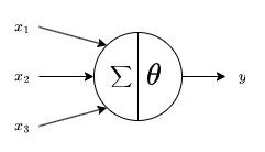
where $\sum$ represents the sum of the input values and $\theta$ represents the threshold.
In this model, the inputs correspond to biological dendrites, the node to the soma and the output to the axon terminal. Unlike synapses in a biological neuron, an MP Neuron does not give different weights to different inputs.
All inputs and outputs are binary. Each input is either excitatory or inhibitory. If any inhibitory input is 1 then the output will be 0 regardless of other inputs. The Rojas diagram for an MP Neuron can be used to represent excitatory and inhibitory inputs
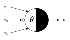
where $\theta$ is the threshold and $x_2$ is an inhibitory input so it has a small circle at the end of the arrow.
The output of MP Neurons can be expressed using vectors. Let $\bm{1} = \begin{bmatrix}1 & 1 & \cdots & 1\end{bmatrix}$ and $\bm{x} = \begin{bmatrix} x_1\\x_2\\\vdots\\x_n\end{bmatrix}$. The sum of the inputs can therefore be expressed as the dot product of these vectors, $z = \bm{1} \cdot \bm{x}$. The threshold can be expressed using a Heaviside function $H_\theta(z) = \begin{cases}1,\quad x \geq \theta\\0,\quad z<\theta\end{cases}$. Therefore, the vector form of the output of the MP Neuron is given by $y = H_\theta(\bm{1} \cdot \bm{x})$.
Logic gates can be emulated using MP Neurons. An MP Neuron for the NOT gate has $\theta = 0$ and an inhibitory input. The Rojas diagram for this neuron is
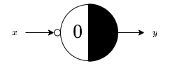
A 2-input AND gate is emulated using a neuron with $\theta = 2$. An $n$-input AND gate is emulated by $\theta = n$. An OR gate is emulated with $\theta = 1$ for any number of inputs.
There are several limitations of the MP Neuron
- Inputs and outputs are limited to binary values only
- All inputs are equally weighted
- The threshold $\theta$ needs to be set manually
Single layer perceptron
The perceptron extends the MP neuron. It can take real numbers as input and each input is weighted. A perceptron is a single-layer neuron and a binary classifier.
A perceptron takes the weighted sum of the input, adds bias and then applies a threshold to determine the binary output.
Perceptron learning works by updating the weights until all nodes are correctly classified.
The vector form of a perceptron consists of a weight vector, $\bm{w}$, and input vector, $\bm{x}$. The weighted sum of inputs including the bias, $b$, is given by $\bm{w} \cdot \bm{x} + b$. The output of the perceptron is given by $y = H(\bm{w} \cdot \bm{x} + b)$. The bias can alternatively be included at the end of the weight vector by adding 1 to the end of the input vector.
The dot product can be used to find the angle between vectors. If the dot product is 0 then the vectors are at right angles, if it is less than 0 then the angle is obtuse and more than 0 is acute.
A node is correctly classified if the angle between it and the weight vector is acute. If a node is misclassified then it can be added to or subtracted from the weight vector. A learning rate hyperparameter which determines the step size at each iteration of training can be used to improve accuracy at the cost of speed.
Multi-layer perceptron
XOR cannot be represented with a single layer perceptron because it is not linearly separable. This can be resolved by either changing the threshold function or using multiple perceptrons. $a \oplus b = (a \cup b) \cap \neg(a \cap b)$ and $\cap, \cup$ and $\neg$ can be emulated with a perceptron so multiple perceptrons can be used to emulate the XOR function. More generally, multiple perceptrons can be combined to recognise more complex subsets of data.
Activation functions
An activation function is a mathematical function attached to each neuron which decides if it should be activated. It adds non-linearity to neural networks and normalises the output of each neuron. The Heaviside function is a simple activation function.
Linear activation functions allow for multiple output values but don't allow for complex relationships with the input.
The sigmoid function, $\sigma(x) = \frac{1}{1+e^{-x}}$ is similar to a step function with a smooth gradient. This allows for more confident classification of inputs and output values are normalised between 0 and 1. The sigmoid function has a vanishing gradient and for very large or small inputs there is almost no change to prediction which inhibits the ability to learn. Another problem is that the sigmoid function is not zero-centred and computationally expensive. The first derivative of the sigmoid function is given by $\sigma'(x) = \sigma(x) \cdot (1-\sigma(x))$.
The $\tanh$ function is given by $$ \frac{e^x-e^{-x}}{e^x+e^{-x}} $$ Unlike the sigmoid function, $\tanh$ is zero centred and output is normalised between -1 and 1. Like the sigmoid function, it still has the vanishing gradient problem and is computationally expensive. This is because the functions are related, $\tanh(x) = 2\cdot\sigma(2x) - 1$. The first derivative of $\tanh$ is given by $\tanh'(x) = 1-\tanh^2(x)$.
The Rectified Linear Unit (ReLU) function is given by $$ \operatorname{ReLU}(x) = \max(0, x) = \begin{cases}x, & x \geq 0\\0, & x < 0\end{cases} $$ The ReLU function is easy to compute and has no vanishing gradient for positive values. The dying ReLU problem occurs when a neuron receives negative input and then only outputs 0. It is also not a zero-centred function.
The leaky ReLU function resolves the dying ReLU problem and is given by $$ \operatorname{LReLU}(x) = \max(\alpha x, x) = \begin{cases}x, & x \geq 0\\\alpha x, & x < 0\end{cases} $$ for some $\alpha$.
Parametric ReLU (PReLU) is a variation of LReLU which makes $\alpha$ a learnable parameter. This is more computationally expensive.
The Exponential Linear Unit (ELU) function is given by $$ \operatorname{ELU}(x) = \begin{cases}x, & x \geq 0\\\alpha(e^x-1), & x < 0\end{cases} $$ This is smoother at $x=0$ than LReLU, does not have the dying ReLU problem and has no vanishing gradient problem for $x \geq 0$. There is still a vanishing gradient problem for $x \leq 0$ and it is more computationally expensive than ReLU and LReLU.
The softmax function is a generalisation of the sigmoid function. It takes as input a vector $z$ of $N$ real values and normalises it into a probability distribution consisting of $N$ probabilities proportional to the exponentials of the input values. $$ y_i = \frac{e^{z_i}}{\sum_{j=1}^Ne^{z_j}} $$ Because this is a probability distribution, $\sum_{i=1}^N y_i = 1$.
The exponential function is needed to account for negative input values as probabilities have to be positive. When $N=2$, the softmax function reduces to the sigmoid function.
The maxout function is a generalisation of ReLU. $$ y = M_k(x) = \max \{w_1x+b_1, w_2x+b_2,\cdots, w_kx+b_k \} $$ where $k$ is the number of affine feature maps, $x$ is the input and $w_i$ and $b_i$ are learnable weights. A single maxout unit can approximately learn any convex function. Two maxout units can approximately learn any continuous function. The maxout function increases the number of hidden neurons and training parameters meaning it is very computationally expensive.
Forward propagation
Forward propagation feeds data forwards through the network. Each hidden layer receives data from the previous layer, processes it and passes it to the next.
The output of a neural network can be computed using either element-wise or by using matrices.
The output at each layer is given by $\bm{z} = f(\bm{w} \cdot \bm{x} + \bm{b})$ where $\bm{w}, \bm{x}$ and $\bm{b}$ are the weights, input and bias for each neuron respectively and $f$ is the activation function.
Vectorisation is an optimisation technique that converts an element-wise operation to one that uses matrices or vectors. Modern CPUs have direct support for vector operations and these are much faster than the element-wise equivalent.
Loss functions and regularisation
A loss function measures the difference between the value predicted by a neural network, $\hat{y}$ and the target value, $y$.
A good loss function
- Is minimised when the predicted value is equal to the target
- Increases when the difference between predicted and target increases
- Is globally continuous and differentiable
- Is convex
The loss function is for a single training input/output pair. The cost function is the average loss function over the entire training set.
There are two groups of loss functions, regression and classification. Regression functions predict continuous, numeric values. Classification functions predict categorical values.
The L1 loss function is given by $L(\hat{y}, y) = |\hat{y} - y|$. This function is intuitive and fast but not differentiable at $\hat{y} = y$ and is less sensitive to outliers. Its cost function is the Mean Absolute Error (MAE) which is given by $\frac{1}{n}\sum_{i=1}^n|\hat{y}_i - y_i|$.
The L2 loss function is given by $L(\hat{y}, y) = (\hat{y}-y)^2$. This function is sensitive to outliers and penalises large errors more strongly but outliers will result in much larger errors. Its cost function is the Mean Squared Error (MSE) which is given by $\frac{1}{n}\sum_{i=1}^n(\hat{y}_i - y_i)^2$.
[missing vector norm stuff]
The L0 norm of a vector is the number of non-zero entries it contains. This is useful for finding the sparsest solution to a set of equations. The L0 norm can be used to limit the number of features to learn from training data which prevents over and underfitting.
Regularisation discourages learning more complex features by applying a penalty to the input parameters with larger weights to avoid the risk of overfitting. Regularisation constrains weights towards 0.
Regularisation using the L0 norm is NP-hard, so L1 and L2 are used instead as these are easier to compute. L1 regularisation is also known as lasso regularisation. L2 regularisation is also known as ridge regularisation.
The log or cross entropy loss function measures the accuracy of a classification model. Log loss compares predicted output $\hat{y}$ with true class $y$ and penalises the probability logarithmically based on how far it diverges from the true class. The log loss function is given by $$ L(\hat{y}, y) = -y\log \hat{y}-(1-y)\log(1-\hat{y}) $$ The $N$-class log loss function is given by $$ L = -\sum_{i=1}^N y_i\log\hat{y}_i $$ with $\sum y_i = 1$ and $\sum \hat{y}_i = 1$.
Backpropagation
Gradient descent is an iterative algorithm that finds a minimal value, $v$, of a function, $f$, given an initial point, $x_0$ such that $$ v = \min_x f(x) $$ Gradient descent works by repeatedly finding $$ x_{t+1} = x_t - \alpha\cdot\nabla f(x_t) $$ where $\alpha$ is a configurable hyperparameter that controls how much the weights are adjusted with respect to the loss gradient.
For example, let $f(x) = x^2 - 2x$, $x_0 = 4$ and $\alpha = 0.4$. The minimum value is given by $$ \begin{aligned} x_1 &= x_0 - 0.4 \times f'(4) = 1.6 \\ x_2 &= x_1 - 0.4 \times f'(1.6) = 1.12\\ x_3 &= 1.02 \\ &\cdots \\ x_n &= 1 \end{aligned} $$ so the minimum value is given by $f(1) = -1$.
For a neural network, gradient descent is used to minimise the loss function. Backpropagation is an effective way of training a neural network by minimising the cost function by adjusting the weights and biases of the network.
The steps to train a neural network are as follows
- Initialise weights and bias at random
- Use forward propagation to compute expected output $\hat{y}$
- Use loss function to measure the error between $\hat{y}$ and target $y$
- Use backpropagation to minimise the loss fiction by adjusting the weights and bias through gradient descent
- Repeat 2-4 until loss function is minimised
Hopfield network
Hopfield networks (HNs) are based on fixed-point iteration, in which an initial guess converges towards the nearest stable fixed point.
Associative learning involves forming associations between items. A HN uses associate memory to associate an input to its most similar memorised output.
Associative memory, also known as Content Addressable Memory (CAM), is the ability to retrieve an item by knowing part of its content.
An $n \times n$ pattern can be represented as a $n^2 \times 1$ vector $\vec{x}$. Each element $x_i$ denotes a state of a neuron $i$. For a discrete HN, each state takes either
- Bipolar values - 1 firing, -1 non-firing
- Binary values - 1 firing, 0 non-firing
The HN is a special form of RNN. It is a single layer, fully connected auto-associative network. Neurons act as both input and output with a binary threshold. HNs are widely used for pattern recognition.
The graph of a HN is a complete graph $G = (V, E)$ where a node $i \in V$ is a perceptron with a state, a pair $(i, j) \in E$ links a pair of nodes with a weight $W_{ij}$. Edges are traversed in both directions and there are no self loops.
The Hebbian learning rules state that
- Neurons that fire together wire together
- Neurons that fire out of sync fail to link
This means simultaneous activation of neurons leads to increased synaptic strength between them.
The weight matrix for a single memorised pattern is given by $$ W = \vec{x} \cdot \vec{x}^T - I $$ $\vec{x} \cdot \vec{x}^T$ is called the rank-one matrix. Subtracting the identity matrix removes the self-loops.
The weight matrix for multiple patterns is given by the average of their weight matrices.
A neuron in a HN has a stable state if the following holds $$ \vec{s}(t+1) = F(W \cdot \vec{s}(t)) $$ where $\vec{s}(t)$ is the state of the HN at time $t$.
For bipolar HN, the activation function is $F = \begin{cases}1 & x \geq0 \\ -1 & x <0 \end{cases}$.
For a memorised pattern $\vec{x}$ to be a fixed-point for the HN it has to satisfy $\vec{x} = F(W \cdot \vec{x})$. A single memorised pattern is always stable.
The energy of a HN is the capacity of the network to evolve. The network will evolve until it arrives at a local minimum in the energy contour. The energy of a HN is given by $$ E = -\sum_{i=1}^n\sum_{j>i}s_i W_{ij}s_j $$ where $s_i$ and $s_j$ are neurons with common weight $W_{ij}$.
The matrix form is given by $$ E = -\frac{1}{2}\vec{s}^TW\vec{s} $$
The energy decreases each time a neuron state changes so $E$ is a decreasing function.
Recurrent neural networks
A Recurrent Neural Network (RNN) is a type of neural network that processes sequential or time series data. RNNs can use their internal state to process variable length sequences of inputs.
Named Entity Recognition (NER) is an information extraction task that locates and classifies named entities in text into pre-defined categories such as names, locations or dates. This is more suited to RNNs than feedforward networks as it makes use of surrounding words for context.
Unlike in a feedforward network, the order of input is important for an RNN.
Elman networks feedback from the internal state output (before weighting the output) to the input. There are weights associated with the input, output and the hidden layer. In Jordan networks the network output (after weighting the output) feeds back to the input.
The output of an Elman RNN is given by $y_t = \sigma(W_o \cdot a_t)$ with $a_t = \tanh(W_i \cdot x_t + W_h \cdot a_{t-1})$ where $W_i$, $W_h$ and $W_o$ are the input, hidden and output weights respectively.
The output of a Jordan RNN is given by $y_t = \sigma(W_o \cdot a_t + b_o)$ with $a_t = \tanh(W_i \cdot x_t + W_h \cdot y_{t-1})$.
Simple RNNs only have a single unidirectional hidden layer. There are several variations
- Deep Recurrent Neural Networks (DRNN)
- Bidirectional Recurrent Neural Networks (BRNN)
- Long Short-Term Memory (LSTM)
- Gated Recurrent Units (GRU)
An RNN can be deep with respect to time and space. A deep RNN is constructed by stacking layers of RNN together. The hidden state information is passed to the next time step of the current layer and the current time step of the next layer.
There are two ways of introducing depth to RNNs
- expanding looping operations into multiple hidden units
- increasing computational depth of a hidden unit
Bidirectional RNNs allow RNNs to have both backward and forward information about the input at every time step.
Simple RNNs are susceptible to the vanishing and exploding gradient problems. For example, a weight of 0.9 after 100 iterations becomes $0.9^{100} = 0.000017\dots$ and a weight of 1.1 becomes $1.1^{100} = 13780.61\dots$. These demonstrate the vanishing and exploding gradient problems respectively. These problems make it difficult for an RNN to capture long term dependencies.
The exploding gradient problem can be reduced by using gradient clipping, where the gradient limited to a threshold value. Vanishing gradient can be reduced using LSTM.
LSTM is a type of RNN which uses three types of gates to control the flow of information passed through the memory cell. The three gates are
- Input gate (i) which controls if data can enter the memory
- Output gate (o) which controls if data can be output from the memory
- Forget gate (f) which controls if all previous data in the memory can be forgotten
$(i_t, o_t, f_t)$ denotes the state of the different gates at time step $t$. When $i_t$ is 1, input is allowed, when it is 0 input is not allowed. $o_t$ allows output when 1, disallow when 0. $f_t$ forgets when 0, remembers when 1.
The equations for LSTM are as follows $$ \begin{aligned} c_t &\leftarrow f_t * c_{t-1} + i_t * a_t\\ a_t &\leftarrow \tanh\left(W \begin{bmatrix} \frac{h_{t-1}}{x_t} \end{bmatrix}\right)\\ h_t &\leftarrow o_t * \tanh(c_t)\\ \begin{bmatrix} f_t \\ i_t \\ o_t \end{bmatrix} &\leftarrow \sigma\left(\begin{bmatrix} W_f \\ W_i \\ W_o \end{bmatrix}\begin{bmatrix} \frac{h_{t-1}}{x_t} \end{bmatrix}\right) \end{aligned} $$ where $c_t$ is the memory state, $a_t$ is the activation value and $h_t$ is the hidden state.
Different RNNs are used for different length inputs and outputs
- One to one
- One to many
- Many to one, can be used for sentiment analysis
- Many to many, can be used for named entity recognition or machine translation
Graph mining
There are several ways of representing graphs
- Adjacency matrix - $(i,j)$ th element is the weight of the edge between $i$ and $j$, requires $O(|V|^2)$ space, ideal for dense graphs, connectivity can be determined in $O(1)$ time, powers of matrix give the number of paths of that length between two nodes
- Laplacian matrix - Given by the degree matrix minus the adjacency matrix, the number of spanning trees in a connected graph is the determinant of any cofactor of the Laplacian matrix, ideal for dense graphs
- Adjacency list - Graph represented as an array of linked lists containing the out-neighbours of each node, requires $O(|E| + |V|)$ space, more efficient for sparse matrices
- Compressed Sparse Row (CSR) - Represents a matrix as a row offset, column index and value
- Coordinate list - Represents a matrix as row index, column index and value
PageRank
PageRank is a ranking algorithm that rates the importance of a webpage recursively based on graph structures. A webpage is considered important if it is pointed to by many important webpages.
A simplified version of PageRank is given by $$ PR(v) = \sum_{x \in I(v)} \frac{PR(x)}{|O(x)|} $$ where $I(x)$ and $O(x)$ are the incoming and outgoing edges of node $x$ respectively.
Simplified PageRank does not work if a node does not have in-neighbours or the graph has cycles.
The Classic PageRank model adds a damping factor $0 \leq c \leq 1$. The algorithm keeps walking with probability $c$ but jumps to another node with probability $1-c$. This prevents the problems with the simplified PageRank algorithm. The Classic PageRank model is given by $$ PR(v) = c\sum_{x \in I(v)}\frac{PR(x)}{|O(x)|} + (1-c)\frac{1}{|V|} $$
The matrix form of PageRank is given by $$ \bm{p} = c\bm{W}\bm{p} + \frac{1-c}{|V|}\bm{1} $$ where $\bm{p}$ is the PageRank vector $\bm{p} = \left[PR(1), \cdots, PR(n)\right]^T$, $\bm{W}$ is a transition matrix and $\bm{1}$ is a vector of 1s.
The transition matrix is given by $$ W_{i,j} = \begin{cases} \frac{1}{|O(j)|} & \text{if } \exists (j, i) \in E \\ 0 & \text{otherwise} \end{cases} $$ The transition matrix is the column normalised adjacency matrix of the graph. This can be denoted $\bm{W} = \bm{A}^T(\bm{D}^{-1})$ where $D$ is the diagonal out-degree matrix.
$\bm{W}$ is column-stochastic because each column sums to 1 and each element is between 0 and 1. $\bm{W}$ describes the transition of a Markov Chain.
The PageRank vector $\bm{p}$ is defined recursively. There are three methods to calculate the PageRank vector
- Fixed-point iteration
- Matrix inversion
- Dominant eigenvector
For fixed-point iteration, let $\bm{p}_ 0 = \frac{1}{|V|}\bm{1}$ and $\bm{p}_ k = c\bm{W}\bm{p}_ {k-1} + \frac{1-c}{|V|}\bm{1}$. $\bm{p_ k} \rightarrow \bm{p}$ as $k \rightarrow \infty$. The number of iterations needed to achieve a desired accuracy $\epsilon$ is given by $k \geq \lceil\log_c(\epsilon/2)\rceil + 1$. The time and space complexity of each iteration is $O(|E| + |V|)$.
Another method is matrix inversion. The PageRank equation can be rearranged to collect $\bm{p}$ on one side $$ \begin{aligned} \bm{p} &= c\bm{W}\bm{p} + \frac{1-c}{|V|}\bm{1}\\ (\bm{I} - c\bm{W})\bm{p} &= \frac{1-c}{|V|}\bm{1}\\ \bm{p} &= \frac{1-c}{|V|}\left(\bm{I} - c\bm{W}\right)^{-1}\bm{1} \end{aligned} $$ This is the closed form of PageRank. The inverse of $\bm{I} - c\bm{W}$ always exists but is expensive to find and very dense. The time and space complexities are $O(|V|^3)$ and $O(|V|^2)$ respectively. This is much slower and uses more space than fixed-point iteration but provides an exact solution.
Another method is using the dominant eigenvector. $||\bm{p}||_1 = 1$ can be rearranged to give $\bm{1}^T\bm{p} = 1$. Multiplying the original equation by 1 gives $$ \begin{aligned} \bm{p} &= c\bm{W}\bm{p} + \frac{1-c}{|V|}\bm{1} \cdot 1 \\ \bm{p} &= c\bm{W}\bm{p} + \frac{1-c}{|V|}\bm{1} \cdot \bm{1}^T\bm{p} \\ \bm{p} &= \left(c\bm{W} + \frac{1-c}{|V|}\bm{1} \cdot \bm{1}^T\right)\bm{p} \end{aligned} $$ The Google matrix $G$ is given by $$ \bm{G}= c\bm{W} + \frac{1-c}{|V|}\bm{1} \cdot \bm{1}^T $$ so the PageRank equation can be expressed as $\bm{p} = \bm{G}\bm{p}$.
HITS
Hyperlink-Induced Topic Search (HITS) is a PageRank-like ranking algorithm that measures the importance of webpages based on authority and hub scores of each webpage. A good webpage should link to other good webpages and be linked by other good webpages.
The authority score $a(x)$ of a node $x$ is given by the sum of the scaled hub scores of its neighbours. The hub score, $h(x)$, is given by the sum of the scaled authority scores of the out-neighbours of $x$.
HITS can be evaluated using three methods
- Iterative
- Dominant eigenvector
- Singular Value Decomposition (SVD)
Graph-based similarity search
Graph-based Jaccard similarity of two nodes $a$ and $b$ is given by $$ \operatorname{sim}(a, b) = \frac{|I(a) \cap I(b)|}{|I(a) \cup I(b)|} $$ where $I(x)$ is the set of incoming neighbours.
Jaccard graph search does not consider the number of common neighbours and does not consider greater than one-hop similarity.
SimRank considers multi-hop neighbours. The SimRank similarity of two nodes $a$ and $b$ is given by $$ s(a,b) = \begin{cases} 0 & \text{if } I(a) = \emptyset \text{ or } I(b) = \emptyset\\ \frac{C}{|I(a)||I(b)|}\sum_{x \in I(a)}\sum_{y \in I(b)}s(x, y) & \text{if } a \neq b\\ 1 & \text{if } a = b \end{cases} $$ where $C$ is a damping factor.
The similarity of all pairs of nodes in a graph is given by $$ \bm{S}_ i = \max\{C \cdot \bm{Q}^T\bm{S}_ {i-1}\bm{Q}, \bm{I}\} $$ where $Q$ is the column-normalised adjacency matrix and $\bm{S}_i$ is the matrix of SimRank values and $\bm{S}_0 = \bm{I}$. The minimum number of iterations needed to achieve accuracy $\epsilon$ is $k\geq \lceil\log_c\epsilon\rceil$.
Dimensionality reduction for time series
Dimensionality reduction reduces the dimension of a data set. This can avoid overfitting, eliminate noise and reduce the amount of space required.
There are three dimensionality reduction techniques
- Piecewise Aggregate Approximation (PAA) - Split the time series into equally sized segments and use the average value for each segment, takes $O(n)$ time for a time series of length $n$
- Piecewise Linear Approximation (PLA) - Approximates each segment of a time series using the best-fit coefficients of the equation of a line
- Adaptive Piecewise Constant Approximation (APCA) - Adaptive PAA, allows for variable length segments
CS349 - Principles of Programming Languages
Lambda Calculus
Lambda calculus consists of constructions of the form $M = x | (\lambda x.M) | (M M)$ where $M$ is a term and $x$ is a variable. These denote variables, abstraction and application respectively. Application is left associative, application binds more tightly than abstraction. $\lambda x.(\lambda y.M)$ can be abbreviated as $\lambda x\;y.M$.
The lambda symbol binds the variable which comes after it. The scope of the binding is the expression that follows the dot.
Free variables are not bound. For example, in $(\lambda x.\lambda y.(xz)(yw)w)$ the free variables are $w$ and $z$ and the bound variables are $x$ and $y$.
The free variables in an expression can be denoted
- $FV(x) = x$
- $FV(\lambda x.M) = M - \{x\}$
- $FV(M_1 M_2) = FV(M_1) \cup FV(M_2)$
A substitution in the term $M$ of the free variable $x$ by the term $N$ is denoted $M[x \leftarrow N]$.
- $x[x \leftarrow N] = N$
- $x[y \leftarrow N] = x$ when $x \neq y$
- $(M_1M_2)[y\leftarrow N] = (M_1[y \leftarrow N] M_2[y \leftarrow N])$
- $(\lambda x.M)[y \leftarrow N] = \lambda x.M$ if $x = y$
- $(\lambda x.M)[y \leftarrow N] = \lambda x.(M[y \leftarrow N])$ when $x \neq y$ and $x$ is not a free variable in $N$
- $(\lambda x.M)[y \leftarrow N] = \lambda z.((M[x \leftarrow z])[y\leftarrow N])$ where $x, y \neq z$ and $z$ is not a free variable in $M$ or $N$.
- Capture avoidance - substitution should not constrain variables unnecessarily
- Freshness - when a variable is not free in $N$ it can't be re-used
- Substitution is a purely syntactic operation in symbols
Alpha equivalence captures the notion that the variable name being bound doesn't matter so the expressions $(\lambda x y z.xxyy)$ and $(\lambda a b c.aabb)$ are equivalent. One expression can be $\alpha$-converted to another using substitution. Expressions that can be $\alpha$-converted to each other are $\alpha$-equivalent.
Beta reduction substitutes an argument into an abstraction, $(\lambda x.M)N \rightarrow M[x \leftarrow N]$, where the left expression is called a beta redex.
- A series of reductions is called a reduction sequence.
- A normal form is where no more reductions are possible.
- An evaluation is $A \Rightarrow B \equiv A \rightarrow^\star B$ where $B$ is a normal form.
- A program is said to diverge when it doesn't terminate.
Eta reduction is a method of simplifying expressions. $\eta$-equivalence is defined as $(\lambda x.Mx) \rightarrow_\eta M$. For example, $(\lambda y. \lambda x. yx)$ is equivalent to $(\lambda y. y)$.
Lambda Calculus is Turing complete.
A normal form is when no further reductions are possible.
- Normal order evaluation reduces the leftmost redex first. If there is a normal form it will be found.
- Applicative order evaluation reduces the rightmost redex first. It is possible that it results in divergence.
Terms are $\beta$-equivalent if they can be reduced to the same normal form. Church's thesis says it is not possible to always prove that two terms are $\beta$-equivalent. This is the incompleteness theorem.
Head normal form is achieved when there are no further useful reductions. A weak normal form does not optimise the body of the function.
Using $e = x | \lambda x. e | e e$, the normal forms ($E$) can be denoted as
- Normal form $E = \lambda x.E | xE_1 \dots E_n$
- Head normal form $E = \lambda x.E | xe_1 \dots e_n$
- Weak normal form $E = \lambda x.e | xE_1 \dots E_n$
- Weak head normal form $E = \lambda x.e | xe_1 \dots e_n$
Any variable or abstraction is in WHNF. An application is in WHNF if it is not a redex.
[ add notes on de bruijn representation ]
Any variable is in normal form. An abstraction is in NF is the body of the abstraction is in NF. An application is in NF if it is not a redex and there is no redex in the sub-expressions.
Some useful combinatory logic lambda expressions are given one letter names
- $I = \lambda x.x$ (Identity)
- $K = \lambda x.\lambda y.x$ (Konstant)
- $Y = \lambda f.(\lambda x.f(xx))(\lambda x.f(xx))$ (Y-combinator)
- $S = \lambda x.\lambda y.\lambda z.xz(yx)$
- $B = \lambda x.\lambda y.\lambda z.x(yz)$ (Composition)
- $T = \lambda x. \lambda y. yx$ (Transposition)
Any combinator can be encoded using only $S$ and $K$.
Church encoding uses the following lambda expressions
- $T = \lambda xy.x$ (True)
- $F = \lambda xy.y$ (False)
- $I = \lambda pxy.pxy$ (If then)
- $A = \lambda pq. pqp$ (And)
- $O = \lambda pq.ppq$ (Or)
- $N = \lambda pab.pba$ (Not)
These lambda functions work like binary operators. For example not true, $N(T)$, evaluates as follows:
- $(\lambda pab.pba)(\lambda xy.x)$
- $\lambda ab . (\lambda xy.x) ba$
- $\lambda ab . b$ which is $\alpha$-equivalent to $F$
There are also definitions for addition and natural numbers
- $add = \lambda ijfx. (if)(jfx)$
- $0 = \lambda fx.x$
- $1 = \lambda fx.fx$
- $2 = \lambda fx.ffx$
- $n \in \mathbb{N} = \lambda fx. f^nx$
For example, $1+1$ is evaluated as follows:
- $(+)(1)(1)$
- $(\lambda ijfx.(if)(jfx))(\lambda fx.fx)(\lambda fx.fx)$
- $\alpha$-equiv to $\lambda ijfx.(if)(jfx))(\lambda gy.gy)(\lambda hw.hw)$
- $(\lambda jfx. ((\lambda gy. gy) f)(jfx))(\lambda hw.hw)$
- $(\lambda fx. ((\lambda gy. gy) f)((\lambda hw.hw)fx))$
- $(\lambda fx . (\lambda y. fy)(fx))$
- $(\lambda fx . ffx)$ which is 2
Environments are associations of free variables with values. For example, $E = {T = \lambda xy.x, O=\lambda pq. ppq, \dots}$. $E \vdash e \rightarrow n$ denotes a judgement and means in a given environment $E$, expression $e$ evaluates to value $n$.
These can be used to write rules, such as $$ \frac{E \vdash e_1 \rightarrow T}{E \vdash O e_1e_2 \rightarrow T} $$ which states that in an environment where $e_1$ evaluates to $T$, we can conclude that $O e_1e_2$ evaluates to $T$.
Another example is for AND: $$ \frac{E \vdash e_1 \rightarrow T \quad e_2 \rightarrow n}{E \vdash A e_1e_2 \rightarrow n} $$
Types can be added to lambda calculus by including the following
- Type environment - List $H = x_1:t_1, \dots x_n:t_n$ of pairs of variables and types, where variables are distinct
- Typing judgement - Triple consisting of a type environment $H$, a term $M$ and a type $t$ such that all the free variables of $M$ appear in $H$ and stating that in the environment $H$, the term $M$ has type $t$, denoted $H \vdash M:t$
- Typing derivations - trees with nodes labelled by typing judgements, giving a demonstration of $H \vdash M:t$
The Simply Typed Lambda Calculus (STLC) consists of
- $x \in$ Variables
- $t ::= o | t \rightarrow t$
- $M ::= x | \lambda x: t.M | MM$
This type system is referred to as System $F_1$.
Dynamic semantics show what a lambda expression evaluates to. Static semantics show what type an expression has.
The natural semantics show the dynamic semantics of a language and are denoted $C \vdash e \Rightarrow v$ where $\Rightarrow$ is the transitive closure of $\beta$-reduction. The rules for application, variables and abstraction are as follows $$ \begin{aligned} &\frac{E \vdash M \Rightarrow \lambda x:t.M' \quad E \vdash M'[x \leftarrow P] \Rightarrow N}{E \vdash MP \Rightarrow N}appl \\ &\frac{}{{x=v, \dots} \vdash x \Rightarrow v} {var}\\ &\frac{E \vdash M \Rightarrow N}{E \vdash \lambda x:t.M \Rightarrow \lambda x:t.N} abs \end{aligned} $$
The rules for types (static semantics) are $$ \begin{aligned} &\frac{H \vdash M: s \rightarrow t \quad H \vdash N : s}{H \vdash MN : t}appl \\ &\frac{}{H, x:t \vdash x:t} {id}\\ &\frac{H,x:s \vdash M:t}{H \vdash \lambda x:s.M:s \rightarrow t} abs \end{aligned} $$
PCF
The PCF language combines Church encoding and type systems. A reduced subset of PCF, PCF-, is defined as $$ \begin{aligned} t ::= \text{num} &| \text{bool} | t \rightarrow t \ M ::= 0 &| \text{true} | \text{false} | \mathbb{N} \ &| \text{succ}(M) | \text{pred}(M) | \text{zero?}(M)\ &| M+M | M \times M \ &| \text{if } M \text{ then } M \text{ else } M | x | \lambda x. t.M | MM \end{aligned} $$
This can be extended with pairs and declarations $$ \begin{aligned} t &::= t * t \ M &::= \left<M, M\right>|\text{fst}(M)|\text{snd}(M) | \text{let } d \text{ in } M\ d &::= x = M | d \text{ and } d \end{aligned} $$
[missing relation between types and values]
Semantic consistency is given by the subject reduction theorems
- If $E \vdash e \Rightarrow v$, $E \in T$ and $T \vdash e: t$ then $v \in t$
- If $E \vdash d \Rightarrow E'$, $E \in T$ and $T \vdash d: T'$ then $E' \in T'$
The Y-combinator is used to represent recursive functions. $Yx = x(Yx)$. There are several ways of representing $Y$ in lambda calculus including $Y = \lambda x.VV$ where $V = \lambda y.x(yy)$ or $Y = ZZ$ where $Z = \lambda zx.x(zzx)$. The factorial function can then be denoted $\text{Fact} = Y(\lambda f: \text{num} \rightarrow \text{num} . \lambda n: \text{num} . \text{if zero?}(n) \text{ then succ}(n) \text{ else} (n \times f(\text{pred}(n))))$.
The shorthand $\mu f. [\dots]$ represents $Y(\lambda f. [\dots])$. PCF also provides other syntactic sugar
- $f = \lambda x.\lambda y. xy$ is written $f(x, y) = xy$
- $f = \mu g. g \dots$ is written $\text{let rec } f = f \dots$
- $\text{let } x = M \text{ in } N$ is written $\text{let } x = M;; N$
Small step semantics can be added to PCF to determine the order of evaluation. The axioms are as follows: [axioms go here]
[call by name?]
[call by value?]
MiniML
The Curry-Howard isomorphism looks at propositions as types. The type of closed expressions can be interpreted as tautologies.
Currying is the technique of transforming a function that takes multiple arguments in such a way that it can be called as a chain of functions each with a single argument.
MiniML has type polymorphism, type inference and variables to refer to unknown types. MiniML consists of terms of the form $$ \begin{aligned} e := & c_\text{bool} | c_\text{num} | \left<e_1,e_2\right> | \text{fst } e | \text{snd } e\ & | x | e_1e_2 | \text{fn } x.e | \text{let } d \text{ in } e\ & | e_1 = e_2 | e_1 + e_2 | \text{if } e_0 \text{ then } e_1 \text{ else } e_2\ & | \text{nil} | e_1 :: e_2 | \text{hd } e | \text{tl } e \end{aligned} $$ and type variables $\tau := \text{num} | \text{bool} | \tau_1 * \tau_2 | \tau_1 \rightarrow \tau_2 | \alpha, \beta,... | \tau \text{list}$.
Polymorphism uses universally quantified types. For a list, nil has type $\forall \alpha.\alpha \text{ list}$ and cons has type $\forall \alpha . \alpha * \alpha \text{ list} \rightarrow \alpha \text{ list}$.
Type inference algorithms
- to each bound variable and to every expression, assign a new type variable
- establish a set of equations
- solve the equations, by replacing variables as needed.
Expressions are unified (denoted $\sim$) by substituting type variables to obtain two identical type expressions. If inconsistent replacements, stop with error.
MiniML type inference works because it is first-order. In order to keep type inference efficient, MiniML keeps types and type schemes separate.
| $\sim$ | $\text{num}$ | $\text{bool}$ | $t_1 \times t_2$ | $t_1 \rightarrow t_2$ | $t_1 \text{ list}$ | $\alpha$ |
|---|---|---|---|---|---|---|
| $\text{num}$ | y | n | n | n | n | $\alpha \leftarrow \text{num}$ |
| $\text{bool}$ | n | y | n | n | n | $\alpha \leftarrow \text{bool}$ |
| $t_3 \times t_4$ | n | n | if and only if $t_1 \sim t_3$ and $t_2 \sim t_4$ | n | n | $\alpha \leftarrow t_3 \times t_4$ |
| $t_3 \rightarrow t_4$ | n | n | n | if and only if $t_1 \sim t_3$ and $t_2 \sim t_4$ | n | $\alpha \leftarrow t_3 \rightarrow t_4$ |
| $t_2 \text{ list}$ | n | n | n | n | if and only if $t_1 \sim t_2$ | $\alpha \leftarrow t_2 \text{ list}$ |
| $\beta$ | $\beta \leftarrow \text{num}$ | $\beta \leftarrow \text{bool}$ | $\beta \leftarrow t_1 \times t_2$ | $\beta \leftarrow t_1 \rightarrow t_2$ | $\beta \leftarrow t_1 \text{ list}$ | $\beta \leftarrow \alpha$ |
Hindley-Damas-Milner type inference algorithm
- Build a tree based on structural induction over the term.
- To each occurrence of a constant, ascribe an arbitrary ‘instance’ of its universally quantified type.
- Build a set of constraints based on each typing statement associated with each rule used in building the tree.
- Solve the constraints to find the most general unifier: two type expressions can be unified if they consist of the same basic type, two type expressions can be unified if one of them is a type variable, two expressions can be unified if they are made of the same type constructor and the sub-expressions can be unified.
[missing loads of stuff]
An abstract data type (ADT) consists of
- content $\left<3, \text{succ}\right>$
- interface $a * (a \rightarrow \text{num})$
- representation $a = \text{num}$
To check the type of an ADT, substitute the representation into the interface to check content.
Imperative languages
The IMP toy language models an imperative language. It consists of
- Arithmetic expressions $a := n|v|a_1+a_2|a_1-a_2|a_1*a_2$
- Boolean expressions $b := \text{true} | \text{false} | a_1=a_2 | a_1 \leq a_2 | ~b|b_1 \wedge b_2$
- Commands $c := \text{skip} | v := a | c_1;c_2 | \text{if } b \text{ then } c_1 \text{ else } c_2 | \text{while } b \text{ do } c$
The language uses a store $s$ which is a mapping from variables to values.
Semantic descriptions are functions that define the meaning of expressions. For example, $A[n]s = N[n]$ means that the semantics of a natural number in a store $s$ is its value. $B[a_1 = a_2] = \lambda s.A[a_1]s = A[a_2]s$ means that the equality operator semantics are the equality of the values of each operand in the store. $B[b_1 \wedge b_2]$ has semantics $B[b_1]s$ is $T$ and $B[b_2]s$ is $T$.
Commands modify stores. Operational semantics show the mapping from commands to stores, $\left<c,s_1\right> \Rightarrow s_2$. The operational semantics of assignment are $\left<v := a, s\right> = s[v \rightarrow A[a]s]$. $\left<\text{skip}, s\right> \Rightarrow s$ means the state is unaffected by skip.
The operational semantics for sequential composition are given by $$ \frac{\left<c_1, s\right> \Rightarrow s_2 \qquad \left<c_2,s_2\right>\Rightarrow s_3}{\left<c_1;c_2, s\right> \Rightarrow s_3} $$
The operational semantics for the if-then-else command are given by $$ \frac{B[b]s \text{ is } T \qquad \left<c_1, s\right> \Rightarrow s_2}{\left<\text{if } b \text{ then } c_1 \text{ else } c_2, s\right> \Rightarrow s_2} $$
and
$$ \frac{B[b]s \text{ is } F \qquad \left<c_2, s\right> \Rightarrow s_2}{\left<\text{if } b \text{ then } c_1 \text{ else } c_2, s\right> \Rightarrow s_2} $$
The operational semantics for the while command are given by $$ \frac{B[b]s \text{ is } T \quad \left<c,s\right> \Rightarrow s' \quad \left<\text{while } b \text{ do } c, s'\right> \Rightarrow s''}{\left<\text{while } b \text{ do } c, s\right> \Rightarrow s''} $$ and $$ \frac{B[b]s \text{ is } F}{\left<\text{while } b \text{ do } c, s\right> \Rightarrow s} $$
Structural operational semantics corresponds to the workings of an abstract machine in executing the first step of a computation, resulting in either a terminal configuration $s'$ or an intermediate configuration $\left<c', s'\right>$.
The structural operational semantics of the while command are given by $$ \frac{B[b]s \text{ is } T}{\left<\text{while } b \text{ do } c, s\right> \rightarrow \left<c; \text{while } b \text{ do } c, s\right>} $$
and $$ \frac{B[b]s \text{ is } F}{\left<\text{while } b \text{ do } c, s\right> \rightarrow s} $$
The structural operational semantics for sequential composition are given by
[missing this]
The derivation sequence of configurations can either be finite, where the last configuration is either a terminal configuration or a stuck configuration, or an infinite sequence. If the derivation sequence from $\left<c, s\right>$ is finite it can be denoted either $\left<c, s\right> \rightarrow^* s'$ or $\left<c, s\right> \rightarrow^* \left<c', s'\right>$.
Block is an extension to IMP which introduces variables with a scope. An example program is
begin var x := 0; var y := 1;
(
    x := 1;
    begin var x := 2; y := x + 1 end;
    x := y + x
)
end
The syntax for commands can be extended to give $c := \dots | \text{begin } d_vc \text{ end}$ and $d_v := \text{var } v := a; d_v | \epsilon$.
Another approach to capturing variable declarations is to make explicit the fact that values are stored in locations. There are environments that map variables to locations and stores that map locations to values. The natural semantics of commands must take the environment into consideration, $E_v \vdash \left<c, s\right> \Rightarrow s'$.
Another extension to the Block language is the Proc language. This adds procedures without parameters. It has the abstract syntax $$ \begin{aligned} c &:= \dots | \text{begin } d_vd_pc \text{ end} | \text{call } p\ d_v &:= \text{var } v := a; d_v | \epsilon\ d_p &:= \text{proc } p \text{ is } c; d_p | \epsilon \end{aligned} $$
This introduces the problem of variable scoping.
[missing scope stuff]
Proc can be extended to add a parameter to procedures, $d_p := \text{proc } p(v) \text{ is } c$.
CS355 - Digital Forensics
Digital forensics is the use of scientific methods to collect probative facts from digital evidence.
Image acquisition
An imaging sensor converts light energy to a proportional electrical voltage. Sensors are usually CCD or CMOS. The sensor array is responsible for sampling. Sampling is how often an image is captured. The grid spacing size in the sensor array determines the spatial resolution of an image. Quantisation is the process of discretisation of intensity values. It converts the continuous signal into one of the discrete values a pixel can have.
Before the imaging sensor there is a colour filter array (CFA). The colour filter only allows particular wavelengths of light through, either red, green or blue. The Bayer pattern is a repeated pattern of filters over four pixels which uses twice as many green filters as red and blue to mimic the human eye, which has twice as many green light absorption cells as red or blue.
CFA interpolation is used to recover the complete RGB values for each pixel in the Bayer pattern. Bilinear interpolation is a popular approach for CFA interpolation.
Human eyes do not perceive light like a camera does. The camera follows a linear relationship between light level and pixel intensity but the human eye does not. Gamma correction is used to account for this, which translates the actual luminance to a perceived luminance according the the sensitivity of the eye to light. For an image with 8 bits per pixel, the pixel values range from 0 to 255. The equation for gamma correction for such an image is $v_{out} = 255 \times \left(\frac{v}{255}\right)^\gamma$. Different values of $\gamma$ will give different results.
A video is a series of images captured at regular intervals. 30 fps is the standard video capture frame rate.
Image representation
The RGB colour model is one of the most common colour spaces used for both acquisition and display. Any point in the RGB color space is a unique combination of red, green and blue.
The Y'UV colour space consists of a luminance component (Y') and chrominance components (U and V). Y'UV was originally developed for adding colour to black and white TV transmissions while providing backwards compatibility.
The YCbCr colour space is a variant of Y'UV. JPEG supports the YCbCr format with 8-bits for each component. YCbCr can be obtained by converting from RGB for each pixel. $$ \begin{bmatrix} Y\\ C_B \\ C_R \end{bmatrix} = \begin{bmatrix} 0.2990 & 0.5870 & 0.1140\\ -0.1678 & -0.3313 & 0.5000\\ 0.5000 & -0.4187 & -0.0813 \end{bmatrix} \begin{bmatrix} R\\G\\B \end{bmatrix} + \begin{bmatrix} 0\\128\\128 \end{bmatrix} $$ This transformation can also be done in reverse from YCbCr to RGB.
Human eyes are much more sensitive to luminance than chrominance so there are redundancies in chrominance channels. The chrominance information can therefore be reduced without noticeable loss of quality. This process is called chroma-subsampling.
The chroma-subsampling scheme is expressed as a three part ratio, A:B:C where
- A is the width of the region in which subsampling is performed
- B is the number of Cb/Cr samples in each row of A pixels (horizontal factor)
- C is the number of changes in Cb/Cr samples between the first and second row (vertical factor)
4:4:4 subsampling preserves the original image. 4:2:2 subsampling merges every two colours into one. 4:2:0 subsampling merges the first two columns into the same colour and the last two into another. This is the most popular format for digital images.
Consider 4:2:0 subsampling on the following full resolution chroma sample $$ \begin{bmatrix} 20 & 22 & 42 & 40\\ 20 & 22 & 43 & 39 \end{bmatrix} $$
There are several techniques for subsampling.
- Average - the average of the original block. For the example, this would be $\begin{bmatrix} 21 & 41\end{bmatrix}$ because the average of $\begin{bmatrix}20 & 22\\20&22\end{bmatrix}$ is 21 and the average of $\begin{bmatrix}42 & 40\\43&39\end{bmatrix}$ is 41.
- Left - the average of the two leftmost chroma pixels of the block, which gives $\begin{bmatrix} 20 & 42\end{bmatrix}$
- Right - the average of the two rightmost chroma pixels of the block, which gives $\begin{bmatrix}22 & 39\end{bmatrix}$
- Direct - the top left chroma pixel, which gives $\begin{bmatrix}20 & 42\end{bmatrix}$
Using 4:2:0 subsampling reduces the size of the chrominance channels by a factor of 4 with little noticeable change in quality.
Examples
Based on 2023 paper, question 1b with additional examples
Consider the chrominance channel $I$: $$ I = \begin{bmatrix} 19 & 20 & 20 & 23 \\ 21 & 22 & 24 & 25 \\ 22 & 22 & 24 & 24 \\ 20 & 20 & 22 & 21 \end{bmatrix} $$
Show the subsampled channel for each of the following formats, using floor to get integer values:
- 4:2:0 left $$\begin{bmatrix}20 & 22 \\ 21 & 23\end{bmatrix}$$
- 4:1:1 direct $$\begin{bmatrix}19 \\ 21 \\ 22 \\ 20\end{bmatrix}$$
- 4:2:2 average $$\begin{bmatrix} 19 & 21\\21 & 24\\22 & 24\\20 & 21\end{bmatrix}$$
- 4:2:0 average $$\begin{bmatrix}20 & 23\\21 & 22\end{bmatrix}$$
- 4:1:1 right $$\begin{bmatrix}21 \\ 24 \\ 24 \\ 21\end{bmatrix}$$
- 4:2:2 direct/left $$\begin{bmatrix}19 & 20\\ 21 & 24\\ 22 & 24\\ 20 & 22\end{bmatrix}$$
2021 paper, question 5b Perform 4:2:2 (average) and 4:2:0 (direct) chroma subsampling on the following matrix. Use floor for integer conversion. $$ M = \begin{bmatrix} 5 & 5 & 0 & 5\\ 5 & 0 & 3 & 2\\ 5 & 5 & 2 & 2\\ 2 & 0 & 1 & 0 \end{bmatrix} $$
- 4:2:2 (average) $$\begin{bmatrix}5 & 2\\2&2\\5&2\\1&0\end{bmatrix}$$
- 4:2:0 (direct) $$\begin{bmatrix}5 & 0 \\5 & 2\end{bmatrix}$$
Comparing images
There are three main methods of comparing the similarity of images
- Mean squared error (MSE), measures dissimilarity
- Correlation, measures similarity
- Structural similarity (SSIM)
The simplest method of measuring similarity is the mean squared error (MSE). The MSE for two images $X$ and $Y$ is defined as $$ MSE(X, Y) = \frac{1}{N}\sum_{i=1}^N(y_i-x_2)^2 $$ where $x_i$ and $y_i$ are pixel values and $N$ is the image size (this requires $X$ and $Y$ to be the same size).
MSE is simple, parameter free, doesn't need memory and has quadratic form meaning it can be optimised easily.
Correlation coefficients measure the statistical relationship between two variables. By modelling an image as a discrete random variable, the mean, variance and standard deviation can be found. For an image $X = \left[x_1, x_2, ..., x_i, ..., x_N\right]$ where $x_i$ is the value of the $i$-th pixel in the image, the mean is given by $$\bar{x} = \frac{1}{N}\sum_{i=1}^Nx_i$$ the variance is given by $$\operatorname{Var}(X) = \frac{1}{N}\sum_{i=1}^N(x_i - \bar{x})^2$$ and the standard deviation is given by $$\sigma(X) = \sqrt{\operatorname{Var}(X)}$$
Covariance measures the relationship between two images $X$ and $Y$ is given by $$ \operatorname{Cov}(X, Y) = \frac{1}{n}\sum_{i=1}^N(x_i - \bar{x})(y_i - \bar{y}) $$
If $X= Y$ then $\operatorname{Cov}(X, Y) = \operatorname{Var}(X)$
The sample correlation coefficient can be computed as $$ r(X, Y) = \frac{\operatorname{Cov}(X, Y)}{\sqrt{\operatorname{Var}(X)\operatorname{Var}(Y)}} = \frac{\operatorname{Cov}(X, Y)}{\sigma(X)\sigma(Y)} $$
Image distortion is caused by structural and non-structural distortions.
Non-structural distortions include
- Luminance change
- Contrast change
- Gamma distortion
- Spatial shift
Structural distortions include
- Noise contamination
- Blurring
- JPEG blocking
- Wavelet ringing
The Structural Similarity (SSIM) index is widely used for benchmarking imaging devices. SSIM compares contrast, luminance and structure to determine image similarity. It is more resistant to image distortions than other methods.
Image enhancement
Image enhancement can be used to improve illumination or contrast, remove noise or sharpen an image. These are useful for forensic applications.
Pixel domain
Pixel/spatial domain processing works directly on pixels in an image. Examples include inversion and gamma correction.
Pixel values in an image can be plotted on a histogram. A high contrast image should ideally have a flat histogram spanning the range of pixel intensities.
Histogram equalisation can be used to enhance contrast in images. Firstly, the histogram has to be normalised into a probability mass function (PMF). Consider a histogram of an image with 64 pixels. A bin with frequency 24 would have probability $24/64 = 0.375$. The PMF is the same shape as the histogram, but the $y$-axis uses probabilities instead of frequencies. Flattening the PMF flattens the histogram. To flatten the PMF, it needs to be converted to a Cumulative Distribution Function (CDF).
For a continuous random variable $X$, the CDF is defined as $F_x(X) = P(X \leq x)$. For a discrete random variable the CDF is $F_x(X) = \sum_{x_i \leq x}{P(X = X_i)}$ or more simply, the sum of probabilities of all bins before it.
To equalise the histogram, the CDF has to be flattened. Each pixel with value $k$ is replaced with $$ \operatorname{round}\left((L-1)\sum_{j=0}^{k}\frac{n_j}{n}\right) $$ where $L$ is the number of pixel values.
For RGB, histogram equalisation can be performed on each RGB channel separately or alternatively the image can be converted to YCbCr and equalisation is done on the luminance channel only.
Histogram equalisation can be generalised to histogram matching. An image histogram can be transformed to other histograms.
Another enhancement is noise removal. Image noise is unwanted structures in an image that degrade its quality. Noise is a random quantity, often unknown. For practical purposes, it is assumed that noise is additive and can be modelled as a random variable of a known distribution function, such as Gaussian noise which follows the Gaussian distribution.
Gaussian noise removal can be done using local averaging. Every pixel value is replaced by the average of its neighbouring pixel values. This reduces noise but causes information loss, causing images to become blurry.
Local averaging is a convolution operation. A 3x3 local averaging mask on a 3x3 section of an image $i_1\dots i_9$ centred on $i_5$ can be expressed as $$ \frac{1}{9} \begin{bmatrix} 1&1&1\\1&1&1\\1&1&1 \end{bmatrix} \begin{bmatrix} i_1&i_2&i_3\\i_4&i_5&i_6\\i_7&i_8&i_9 \end{bmatrix} $$ where the left part is called the kernel, filter or weights.
Salt and pepper noise is usually caused by faulty sensors. Only a few pixels are modified and replaced by black or white. This type of noise can be removed with a median filter, which takes the median of neighbouring pixels.
Frequency domain
Two methods to transform an image from the pixel domain to the frequency domain are
- 2D Discrete Fourier Transform (DFT)
- 2D Discrete Cosine Transform (DCT)
Any function can be expressed in terms of harmonic functions of different frequencies. A discrete function with length $M$ can be represented as the sum of harmonic functions $$ f(x) = \sum_{u=0}^{M-1}F(u)e^{\frac{2\pi iux}{M}} $$ As an orthonormal basis this is $$ f(x) = \sum_{u=0}^{M-1}F(u)\frac{1}{\sqrt{M}}e^{\frac{2\pi iux}{M}} $$ where $F(u)$ is a Fourier coefficient.
This can be represented using matrices $$ \begin{bmatrix} f(0)\\ f(1)\\f(2) \\ \vdots \\ f(M-1) \end{bmatrix} = \frac{1}{\sqrt{M}} \begin{bmatrix} 1 & 1 & 1 & \cdots & 1\\ 1 & e^{\frac{2\pi i}{M}} & e^{\frac{4\pi i}{M}} & \cdots & e^{\frac{2(M-1)\pi i}{M}} \\ 1 & e^{\frac{4\pi i}{M}} & e^{\frac{8\pi i}{M}} & \cdots & e^{\frac{4(M-1)\pi i}{M}} \\ \vdots & \vdots & \vdots & \ddots & \vdots \\ 1 & e^{\frac{2(M-1)\pi i}{M}} & e^{\frac{4(M-1)\pi i}{M}} & \cdots & e^\frac{2(M-1)^2\pi i}{M} \end{bmatrix} \begin{bmatrix} F(0) \\ F(1) \\ F(2) \\ \vdots \\ F(M-1) \end{bmatrix} $$ This is called the inverse Fourier transform and transforms frequency into space/time. The forward transform is found by taking the conjugate transpose, which transposes the matrix and negates the imaginary parts of the exponents: $$ \begin{bmatrix} F(0) \\ F(1) \\ F(2) \\ \vdots \\ F(M-1) \end{bmatrix} = \frac{1}{\sqrt{M}} \begin{bmatrix} 1 & 1 & 1 & \cdots & 1\\ 1 & e^{\frac{-2\pi i}{M}} & e^{\frac{-4\pi i}{M}} & \cdots & e^{\frac{-2(M-1)\pi i}{M}} \\ 1 & e^{\frac{-4\pi i}{M}} & e^{\frac{-8\pi i}{M}} & \cdots & e^{\frac{-4(M-1)\pi i}{M}} \\ \vdots & \vdots & \vdots & \ddots & \vdots \\ 1 & e^{\frac{-2(M-1)\pi i}{M}} & e^{\frac{-4(M-1)\pi i}{M}} & \cdots & e^\frac{-2(M-1)^2\pi i}{M} \end{bmatrix} \begin{bmatrix} f(0)\\ f(1)\\f(2) \\ \vdots \\ f(M-1) \end{bmatrix} $$ This is called the forward Fourier transform and transforms time/space into frequency.
The 1D Fourier transform can be extended to the 2D Fourier transform. An $M \times N$ image can be expressed as $$ f(x,y) = \sum_{u=0}^{M-1}\sum_{v=0}^{N-1}F(u,v)e^{2\pi i\left(\frac{ux}{M} + \frac{vy}{N}\right)} $$
The 2D DFT is given by $$ F(u, v) = \frac{1}{M}\frac{1}{N}\sum_{x=0}^{M-1}\sum_{y=0}^{N-1}f(x,y)e^{-2\pi i\left(\frac{ux}{M} + \frac{vy}{N}\right)} $$
Most noise is found in high frequency components of an image. Removing high frequency coefficients in the frequency domain can remove noise in the pixel domain but does mean some information is lost.
Different masks can be applied to the frequency domain for noise removal
- Ideal
- Gaussian
- Butterworth
These filters can be either high or low pass to remove high or low frequencies.
Notch filters can be used to remove repetitive spectral noise from an image.
The Discrete Cosine Transform (DCT) is similar to DFT. It uses cosines as a basis instead of harmonic functions. The forward 1D DCT is given by $$ F(u) = \sum_{x=0}^{N-1} f(x)\alpha(u)\cos\left[\frac{\pi(2x+1)u}{2N}\right] $$ and the inverse DCT is given by $$ f(x) = \sum_{u=0}^{N-1} F(u)\alpha(u)\cos\left[\frac{\pi(2x+1)u}{2N}\right] $$ where $\alpha(u) = \begin{cases}\sqrt{\frac{1}{N}} \text{ for } u = 0\\\sqrt{\frac{2}{N}} \text{ otherwise}\end{cases}$
The forward and inverse transforms have the same basis and the basis is orthonormal, real and symmetric.
The DC component is given by $F(u = 0)$ which simplifies to $$ \frac{1}{\sqrt{N}}\sum_{x=0}^{N-1}f(x) $$
The 2D DCT is given by $$ F(u, v) = \sum_{x=0}^{M-1}\sum_{y=0}^{N-1}f(x,y)\alpha(u)\alpha(v)\cos\left[\frac{\pi(2x+1)u}{2M}\right]\cos\left[\frac{\pi(2y+1)v}{2N}\right] $$ and the DC component is given by $$ \frac{1}{\sqrt{MN}} \sum_{x=0}^{M-1}\sum_{y=0}^{N-1} f(x,y) $$ DCT is ideal for compression because values can be discarded without noticeable loss of image quality.
Digital watermarking
Digital watermarking inserts a signature pattern into data before it is distributed. There are several types
- Blind - doesn't require original data to recover the watermark
- Visible - claim image ownership
- Private - can only be detected by authorised persons
- Robust - resistant to cropping, rotation or resizing
Pixel domain
One method of watermarking is bitplane substitution. A bitplane is the value of the a specific bit of each pixel in an image. The LSB bitplane is every least significant bit in the image. The LSB bitplane has the least effect on the image when replaced with a watermark so can be used for invisible watermarking. Using higher significance bitplanes makes the watermark more visible. Watermarks can either be unrelated images or be derived from the original image.
Bitplane substitution is simple and fast, allows for visible or invisible watermarks and does not necessarily require the original image to recover the watermark but is fragile and vulnerable to cropping.
Frequency domain
Watermarking can be done in the frequency domain by altering components of the DCT or DFT of an image. This makes invisible watermarks which are more robust to common attacks.
The DCT basis can be divided into low, mid and high frequency regions. The low and mid frequency regions are perceptually important so are used for watermarking. The watermark can then be embedded using LSB substitution or spread spectrum watermarking.
Spread spectrum (SS) watermarking uses a random, Gaussian-distributed sequence as a watermark. This watermark can then be embedded into the perceptually important DCT coefficients. For coefficients $h$ and watermark $w$, the watermarked coefficients $h^*$ can be obtained using several methods such as
- $h^* = h(1+\alpha w)$
- $h^* = h(e^{\alpha w})$
- $h^* = h(1+\alpha hw)$
where $\alpha$ is some constant. Higher values of $\alpha$ cause more distortion to the watermarked image.
Hybrid watermarking uses a combination of pixel and frequency domain watermarking on blocks in an image.
Watermarking in the frequency domain is more robust to cropping, compression, removal and filtering than in the pixel domain.
Recovered watermarks can be compared to the original watermark. For pixel domain watermarking, MSE, correlation or SSIM can be used. For spread spectrum, the similarity is given by $$ \operatorname{sim}(\hat{w}, w) = \frac{\hat{w}w^T}{\sqrt{\hat{w}\hat{w}^T}} $$ where $w$ is the original watermark and $\hat{w}$ is the recovered watermark.
Attacks on watermarks include
- Compression
- Filtering
- Jitter attack - randomly duplicates and deletes visually imperceptible data
Compression
Raw images have lots of redundant data. Both lossless and lossy compression can be applied to images. Types of redundancy include
- Spatial - neighbouring pixels have very similar values
- Psychovisual - details in images humans can't see
- Coding - an image can be represented using a lower bit depth
JPEG is the most common image compression algorithm. It has the following steps
- Colour space conversion - Convert RGB to YCbCr, chrominance channels can be subsampled
- Division into sub-images - Divide image into non-overlapping blocks called macroblocks or minimum encoded units, blocks are usually 8x8 or 16x16
- DCT on each block
- Quantiser - apply matrix that roughly models the human sensitivity to the different DCT coefficients, different matrices are used for different image qualities, results in lots of 0 coefficients
- Huffman coding - efficiently and losslessly encode quantised DCT coefficients
Compression-based forensics
Compression-based forensic techniques rely mostly on detecting artifacts introduced by multiple quantisation.
One technique is double compression detection. Quantisation changes DCT coefficients so double quantisation artifacts will be visible in the distribution of DCT coefficients. Quantisation can be expressed as $q_a(u) = \left\lfloor\frac{u}{a}\right\rfloor$ where $a$ is the quantisation factor. De-quantisation is given by $q_a(u)a = \left\lfloor\frac{u}{a}\right\rfloor a$ and double quantisation is given by $q_{ab}(u) = \left\lfloor q_a(u)\frac{a}{b}\right\rfloor = \left\lfloor\left\lfloor\frac{u}{a}\right\rfloor\frac{a}{b}\right\rfloor$.
The histograms of the DCT coefficients can be analysed to look for quantisation artifacts. Periodic empty bins or periodic peaks in the histogram are likely double quantisation artifacts.
Another technique is JPEG ghost detection. By looking at how the quantisation error changes when using different quantisation factors it is possible to see artifacts where different quantisation factors were used for different parts of an image.
Copy-move forgery
Copy-move forgery involves copying part of an image to another part of the same image. It can be detected using several methods
- Exhaustive search by circular shift and match
- Block matching in the pixel or frequency domains
Exhaustive search works by repeatedly circular shifting the image and looking for matching segments. Erosion and dilation are used to reduce false positives. Exhaustive search is computationally expensive.
Block matching works by converting blocks in an image to vectors and searching for matches. In the spatial domain, the block matching algorithm is as follows
- Slide a $b \times b$ block along the image from top left to bottom right
- Convert each block into a vector of length $b^2$ along with its position to form the feature table
- Sort the feature table lexicographically, identify consecutive similar rows as these correspond to similar blocks
- Identify the position of the similar blocks
This can also be done in the frequency domain using blocks of DCT coefficients. Lexicographical sorting in the pixel domain mainly considers the first pixel in a block which might not be representative of the whole block whereas in the frequency domain blocks are sorted by their DC component which contains the most information about the block and can produce better results.
Feature matching
Image features can also be used for forgery detection. Image features can be global or local depending on whether they capture properties of the entire image or a smaller part of it. Features can be pixel values, features in the frequency domain, statistical features or features that encode shape, colour or texture. A good feature should be a compact and robust against geometric and photometric distortion.
Local binary pattern (LBP) is a feature that can efficiently encode the texture information of an image region. It considers the values of neighbouring pixels to identify patterns. Rotation invariant LBP considers the LBP at different rotations and takes the minimum.
An LBP histogram can be used to detect copy-move forgery. The histogram uses a bin for each LBP value which isn't compact, so a more compact representation uses bins for each uniform LBP value and a bin for non-uniform LBP values. A value is uniform if there are at most 2 changes in bit from left to right. For example, 11101111 (2 changes) is uniform but 01101001 (5 changes) is not.
The gradients, $G$ of an image are given by $$ G_x = \nabla f_x * f(x, y)\\ G_y = \nabla f_y * f(x, y) $$ where $*$ denotes convolution and $$ \begin{aligned} \nabla f_x &= \begin{bmatrix} 1 & -1 \end{bmatrix} \text{ or } \begin{bmatrix} -1 & 1 \end{bmatrix} \\ \nabla f_y &= \begin{bmatrix} 1 \\ -1 \end{bmatrix} \text{ or }\begin{bmatrix} -1 \\ 1 \end{bmatrix} \end{aligned} $$ for forward and backward difference respectively.
The magnitude is given by $G_{mag} = \sqrt{G_x^2 + G_y^2}$ or $G_{mag} = |G_x| + |G_y|$ and the direction is given by $G_{ang} = \tan^{-1}\left(\frac{G_y}{G_x}\right)$.
$G_{mag}$ and $G_{ang}$ are used to produce a histogram where each bin is an angle. This is called a Histogram of Oriented Gradients and can be used like the LBP histogram to detect features.
Source Device Identification
Source device identification considers two problems
- Verification - verifies if a given image was captured by a given device
- Recognition - determines which device captured an image
Source device identification can be done using the following
- Chrominance subsampling (only useful if different devices use different subsampling methods)
- EXIF header - camera model, exposure, date/time, resolution (may be removed)
- Watermarking - some camera models embed invisible watermarks for device identification
- Sensor Pattern Noise (SPN) - imperfections and noise characteristics of imaging sensors
SPN is intrinsic to the image acquisition process so can't be avoided and is resistant to image processing such as JPEG compression.
Sensor noise consists of shot noise and SPN. Shot noise is random noise caused by the number of photons collected by a sensor and can be modelled as a Poisson distribution. SPN is a deterministic distortion component and stays approximately the same over multiple images.
SPN can be divided into Fixed Pattern Noise (FPN) and Photo-response Non-Uniformity (PRNU). PRNU can also be divided into Pixel Non-Uniformity (PNU) and low frequency defects.
FPN refers to the variation in pixel sensitivity when a sensor array is not exposed to light. It is also called the dark current noise. FPN can be suppressed by subtracting a dark image taken by the same sensor from a given image.
PRNU is the dominant component of SPN. The primary part is PNU which arises from the different sensitivity of pixels to light. This is caused by properties of silicon and manufacturing imperfections. PNU is not affected by temperature or other external conditions. PNU is unique and can be used for source device identification.
Low frequency defects are caused by light refraction from dust and optical surfaces.
Sensor noise can be modelled as $$ y_{ij} = f_{ij}(x_{ij}+\eta_{ij}) + c_{ij} + \epsilon_{ij} $$ where $y$ is the pre-processed pixel output, $f$ is PRNU, $x$ is the light level of the $ij$ th sensor, $\eta$ is shot noise, $c$ is FPN and $\epsilon$ is random noise.
The PRNU can be found by ignoring shot noise and random noise and rearranging $$ f_{ij} = \frac{y_{ij} - c_{ij}}{x_{ij}} $$ but the pre-processed pixel value, $y_{ij}$ is not available so estimation has to be used instead.
SPN can be approximated using multiple reference images. The scene content can be suppressed from each image by de-noising and then subtracting the de-noised image from the original image to get the noise residual. The average noise residual over all the images gives a reference estimate for the SPN.
The SPN of a single test image can be estimated by assuming no post-processing takes place, giving $SPN_{ij} = y_{ij} - F(y_{ij})$ where $F$ is a de-noising filter. Rearranging the sensor noise model and ignoring FPN and random noise gives $SPN_{ij} = f_{ij}(x_{ij}+\eta_{ij}) - F(f_{ij}(x_{ij}) + \eta_{ij})$. Assuming the filtered image is similar to the original, this can be rewritten as $SPN_{ij} = f_{ij}(x_{ij}+\eta_{ij}) - f_{ij}(\hat{x}_ {ij} + \hat{\eta}_ {ij})$ which can be rewritten as $SPN_{ij} = f_{ij}(\Delta x_{ij} + \Delta \eta_{ij})$ where $\Delta x_{ij}$ is the high frequency scene details and $\Delta \eta_{ij}$ is the shot noise residual.
Video forensics
As videos are just sequences of images, the same forgeries occur and the same forensic techniques can be applied to detect them.
One type of video-specific forgery is frame deletion. This can be detected through analysis of prediction errors.
Instead of analysing each frame in a video, small groups of frames are intracoded into a single image called an I-frame or keyframe. Frames predicted from I-frames are called P-frames. B-frames are predicted from both I- and P-frames. The difference between a real and predicted frame is called an error frame.
Video frames are divided into a sequence of groups of pictures which are encoded and decoded independently.
CS435 - Advanced Computer Security
Computer security is the protection of items of value, called assets. These items include software, hardware and data.
A vulnerability is a weakness in the system that could be exploited to cause harm. A threat is a set of circumstances that has the potential to cause loss or harm. Control or countermeasures are used to prevent threats becoming vulnerabilities.
Security focuses on the CIA triad
- Confidentiality - Prevention of unauthorised disclosure of information
- Integrity - Detection of unauthorised modification of information
- Availability - Authorised users should not be prevented from accessing assets when required
Other security requirements include
- Authentication - Something you know, have or are
- Non-repudiation - Cannot deny doing something
Threats can be grouped into natural and human causes. Human threats can be either benign or malicious. Malicious threats can be random or directed.
Security engineering is about building systems to remain dependable in the face of malice, error or mischance.
The weakest link property states "A security system is only as strong as its weakest link". This is why security systems are so hard to get right.
Users and security
Users should be assumed to be somewhat careless, incompetent and dishonest. Many real attacks exploit psychology as much as technology, such as phishing.
Some psychological errors are
- Capture error - An error where more frequent, practised behaviour takes place when a similar but less familiar was intended
- Post-completion error - Once an immediate goal is completed, people are easily distracted from lesser but still important tasks, like leaving your card after getting cash from an ATM
Captchas are a spam-prevention method that are supposed to be solvable by humans and not computers but computers are getting better at them.
Classical cryptography
Cryptanalysis is the process of analysing weaknesses of cipher algorithms. There are four general types of attack
- Ciphertext only - The attacker only has a ciphertext
- Known-plaintext - The attacker has a known plaintext and its corresponding ciphertext
- Chosen-plaintext - The attacker can obtain ciphertexts for any plaintext
- Chosen-ciphertext - The attacker can decrypt any ciphertext
The two basic principles to obscure redundancies in a plaintext message are
- Confusion - Obscures the relationship between plaintext and ciphertext, such as substitution
- Diffusion - Dissipates the redundancy of the plaintext by spreading it out over the ciphertext, such as transposition
Substitution ciphers can be monoalphabetic, where one character always maps to another, or polyalphabetic, where different mappings are used for each character.
The Caesar cipher is a monoalphabetic cipher. It works by shifting the alphabet some number of positions. ROT13 is another monoalphabetic cipher which shifts the alphabet by 13 characters.
Suppose $a$ and $b$ are integers and $m$ is a positive integer. If $m$ divides $b-a$, this is denoted $a \equiv b (\mod m)$. This is called a congruence and is read $a$ is congruent to $b$ modulo $m$. $m$ is called the modulus.
Shift ciphers are not secure because they can be broken by exhaustive search. There are only 26 possible keys and for a cipher to be secure the key space must be very large.
Substitution ciphers have a large key space but are not secure because they only provide confusion so are susceptible to frequency analysis. A secure cipher should combine both confusion and diffusion.
The Vigenère cipher is a polyalphabetic cipher based on the idea of combining a few Caesar ciphers into one. The cipher can be broken in two steps: finding the key length and finding each letter of the key.
The key length can be found using the Kasiski method by looking for repeated ciphertext phrases and using the distance between them to determine the key length. If the distance between is 15, for example, the key length would be 3, 5 or 15.
Another method to find the key length is using the index of coincidence. Suppose $x = x_1x_2 \dots x_n$ is a string of $n$ characters. The index of coincidence of $x$ is defined to be the probability that two random elements of $x$ are identical. The index of coincidence can then be calculated for different key lengths until a value similar to that of normal text is found.
Once the key length is known, each character of the key can be solved like the Caesar cipher using exhaustive search.
Stream ciphers
A stream cipher works by encrypting data one byte at a time.
A one-time pad (OTP) is a simple stream cipher with perfect security. It works by XORing the plaintext with a key of the same length. This key must be random, the same length as the plaintext and used only once, so this is not very useful in practice.
The OTP was believed to be unbreakable but there was no proof until Shannon developed the concept of perfect secrecy.
A cryptosystem has perfect secrecy if $P(m|c) = P(m)$ for all $m \in M$ and $c \in C$ where $M$ is the message space and $C$ is the ciphertext space.
The one-time pad can therefore be proven to have perfect secrecy: $$ \begin{aligned} P(m|c) &= \frac{P(c|m)P(m)}{P(c)} \text{ (Bayes' theorem)}\\ P(c|m) &= P(m \oplus k|m) = P(k) = \frac{1}{|K|}\\ P(c) &= \sum P(m_i)P(k_i) = \frac{1}{|K|}\sum P(m_i) = \frac{1}{|K|}\\ P(m|c) &= \frac{\frac{1}{|K|}P(m)}{\frac{1}{|K|}} = P(m) \blacksquare \end{aligned} $$ where $K$ is the key space.
Stream ciphers can use a short secret key to generate a long key stream. Synchronous stream ciphers use a linear recurrence to generate the key stream. This type of key stream can be efficiently implemented in hardware using a linear feedback shift register (LFSR).
One attack on shift ciphers is using the same key twice. Due to the properties of XOR, if the same key is used for two messages the ciphertexts can be XOR'd to get the XOR of the plaintext, from which the original messages can be worked out.
Another limitation of stream ciphers is that they do not provide integrity. Part of a message can be XOR'd without knowing the key to change the original message.
Block ciphers
A block cipher works by encrypting blocks of data.
A pseudo-random function (PRF) is defined as $F: K \times X \rightarrow Y$ where $K$ is the key, $X$ is the input and $Y$ is the output. There must exists an efficient algorithm to evaluate $F(k, x)$.
A pseudo-random permutation (PRP) is defined as $E: K \times X \rightarrow X$ such that there exists an efficient deterministic algorithm to evaluate $E(k, x)$, the function $E(k, \cdot)$ is one-to-one and there exists an efficient inversion function.
DES is a Feistel cipher. A Feistel cipher can use the same hardware for encryption and decryption. In the forward direction, $L_{i+1} = R_i$ and $R_{i+1}=L_i \oplus F(K_i, R_i)$. In the reverse direction, $R_i = L_{i+1}$ and $L_i = R_{i+1} \oplus F(K_i, L_{i+1})$ where $L$ and $R$ are the left and right blocks respectively and $F$ is the Feistel function.
By not swapping the blocks after $n$ rounds, the encryption of $L_0R_0$ produces $R_nL_n$ as output. This can be input to the same hardware for decryption to give $L_0R_0$ as desired.
The Feistel function for DES expands the block to 48 bits, then XORs it with the 48 bit round key. This is then passed through 8 substitution boxes (S-boxes) to give a 32 bit output. This is then permuted to give the final output.
The 56 bit key size for DES is too weak and can be brute forced with modern hardware. Double DES uses 2 keys and encrypts the input twice. This only offers 57 bits of security compared to 56 bits for DES, meaning it is ineffective. Triple DES uses 3 keys for 112 bits security. Triple DES is still considered secure.
AES is the successor to DES. It uses 128-bit blocks and key sizes of 128, 192 or 256-bits. AES is based on a substitution-permutation network instead of a Feistel network. AES uses 3 methods - SubBytes, ShiftRows and MixColumns.
Suppose $p$ is a prime. $Z_p$ is a field. $Z_7 = {0,1,2,3,4,5,6}$. Given two prime elements, $a = 3$ and $b=5$ for example, $a \times b \mod 7 = 1$. $b$ is the multiplicative inverse of $a$. Given $a$, $b$ can be calculated using the extended Euclidean algorithm. AES uses a finite field called a Galois field $GF(2^8)$ which works on polynomials. For example, 5 in the field is $x^3 + 1$, which corresponds to the binary representation of 5, 1001. Irreducible polynomials are polynomial representations of prime numbers.
Elements can be multiplied in a finite field by multiplying their polynomials and finding the modulus by an irreducible polynomial.
SubBytes takes an element of $GF(2^8)$ as input, finds the multiplicative inverse and then applies an affine transform to get the substituted value. Unlike DES, the substitution is not random and does not need to be hardcoded.
ShiftRows shifts the bytes in the last three rows of the state. MixColumns multiplies each column by a set polynomial to mix the columns. The key is expanded to provide the key schedule used in each round of encryption.
Different number of rounds are used depending on key size. 128 uses 10 rounds, 192 uses 12 and 256 uses 14. The key scheduling algorithm is different for 256-bit keys.
AES can be used in different modes of operation.
- Electronic Code Block (ECB) - Divide plaintext into blocks, encrypt each block and concatenate. If the same block is encrypted it has the same output so patterns can be found at the block level and should not be used in practice.
- Cipher Block Chaining (CBC) - An initialisation vector (IV) is used which is XOR'd with the first block, then the output of each block is XOR'd with the plaintext of the next. This is one of the most widely used modes. Decryption can be parallelised, but encryption can not. The random IV means the same input gives different outputs. If one plaintext block is changed, all subsequent blocks will be affected.
- Cipher Feedback Mode (CFM) - Turns a block cipher into a stream cipher encrypting the IV, which can then be XORd with the plaintext a byte at a time to give the ciphertext. Once an entire block of ciphertext is produced, it is encrypted and then XORd with the next plaintext block byte by byte. If a byte is lost the ciphertext can't be decrypted. Encryption can't be parallelised but decryption can.
- Output Feedback Mode (CFB) - Also a stream cipher, but the encrypted IV is encrypted in the next round instead of the first ciphertext block. The encryption and decryption operations are the same.
- Counter Mode (CTR) - A counter is encrypted each round, the result of which is XORd with the plaintext. This also works as a stream cipher, encryption and decryption are the same and, unlike CBC, both can be parallelised.
If plaintext is not evenly divisible by the block size it needs to be padded. Padding can be generated with algorithms like PKCS7 where each byte of padding is the number of bytes of padding, so 4 byte padding would be 0x04 0x04 0x04 0x04. The padding needs to be removed after decryption. If an error is found in the padding after decryption, it can be concluded the key or IV was wrong. The padding oracle attack uses invalid padding errors from a server to recover a plaintext.
Padding oracle attack
Consider an attacker which has intercepted a 64-byte encrypted message and a server which returns a padding error if the message it receives doesn't have correct padding (the padding oracle). The attacker can send the oracle as many messages as they like. Suppose the ciphertext is $c_1c_2\dots c_{64}$ and the plaintext is $p_1p_2\dots p_{64}$ where each $c_i$ and $p_i$ are a byte. Suppose the block size of the cipher is 16 bytes. When decrypting the final block of a message, bytes $c_{49}\dots c_{64}$ are put through the decryption cipher to give $d_{49} \dots d_{64}$, which is then XORd with the penultimate ciphertext block $c_{33} \dots c_{48}$.
The attacker can try changing last byte of the penultimate ciphertext block, $c_{48}$, to every value (0 to 255) and sending it to the oracle. The attacker will get a padding error for every value except one, denoted $c^\prime_{48}$, which causes $p_{64}$ to be 0x01, as this is the only value that would be valid padding.
By the definition of CBC, $p_{64} = d_{64} \oplus c_{48}$. It is also true that $d_{64} = p_{64} \oplus c_{48}$ by the properties of XOR.
Once the attacker has found $c^\prime_{48}$ such that $p_{64}$ is 0x01, they can find the original value of $p_{64}$ with the two equations above because 0x01 $= d_{64} \oplus c^\prime_{48}$ and $d_{64} = p_{64} \oplus c_{48}$. Combining these gives 0x01 = $(p_{64} \oplus c^\prime_{48}) \oplus c_{48}$, which can be rearranged to $p_{64} = (c_{48} \oplus c^\prime_{48}) \oplus $ 0x01. The attacker knows $c_{48}$ from the original intercepted message and $c^\prime_{48}$ from the trial and error with the padding oracle, so has all the information they need to work out $p_{64}$, the final byte of the plaintext.
To get the next byte of plaintext, the padding will need to be 0x02 0x02. Let $c^{\prime\prime}_ {48}$ denote the value of $c_ {48}$ needed to make $p_ {64} = $ 0x02. Because $p_ {64}$ and $c_ {48}$ are known, $c^{\prime\prime}_ {48}$ can be determined without trial and error. The attacker wants $c^{\prime\prime}_ {48} \oplus d_ {64}$ = 0x02 which can be rearranged to $c^{\prime\prime}_ {48} = (c_ {48} \oplus p_ {64}) \oplus$ 0x02, which are all known values. Then the attacker has to try every value of $c_ {47}$ until the oracle doesn't give a padding error. The same calculation can be used to find $p_ {47}$. This can then be repeated for every byte in the block.
It is not possible to have more than one block of padding, so after the first block is found, $c_{49}\dots c_{64}$ are not included in the ciphertext any more when breaking the next block. This can then be repeated for every block until the entire plaintext is found.
The padding oracle attack can be prevented by providing a more generic error, although this is still vulnerable to timing attacks if the server rejects invalid padding quicker than other errors.
A hash function compresses an arbitrary message into an output of fixed length. Cryptographic hash functions are those suitable for cryptographic use.
A hash function, $H$, has three security requirements
- Pre-image resistance - Given $H(m)$ it is infeasible to find $m$
- Second pre-image resistance - Given $m_1$, it is infeasible to find a different message $m_2$ such that $H(m_1) = H(m_2)$
- Collision resistance - Infeasible to find two messages $m_1$ and $m_2$ such that $H(m_1) = H(m_2)$
The birthday paradox refers to the counterintuitive fact that a group of only 23 people are needed such that the probability that two people share the same birthday exceeds 50%.
The birthday attack on collision resistance uses the birthday paradox to find collisions. The attacker selects $2^{n/2}$ random input messages where $n$ is the hash function output length and computes the hash of each input message until a collision is found. The consequence of this is that for $n$-bit security, a hash function must have an output of at least $2n$ bits.
Collisions in a hash function for digital signatures is dangerous because it allows for producing counterfeit signatures.
A typical hash function involves three components in the design
- Operation mode
- Compression function structure
- Confusion-diffusion operations
The Merkle-Damgård construction is a method of building collision-resistant hash functions from a collision-resistant one-way compression function.
The Davies-Meyer compression function uses a block cipher. For a message consisting of $n$ blocks, $m_1\dots m_n$, each block of the hash output, $H_i$, is the previous hash block $H_{i-1}$ encrypted with $m_i$ as the key XORd with $H_{i-1}$, that is, $H_i = E_{m_i}(H_{i-1}) \oplus H_{i-1}$. This is a compression function because the input is (key size + block size) and the output is just (block size).
SHA256 uses the Merkle-Damgård construction with the Davies-Meyer compression function and the SHACAL-2 block cipher.
Hash functions can be used for
- Digital signatures
- Data integrity
- Random number generation
- Data privacy
- Commitment scheme
- Blockchains
Hashing can be used to securely store passwords but are vulnerable to dictionary attacks unless a salt is used, but this is still vulnerable to brute force attack as passwords have low entropy.
Message integrity can be ensured by adding a Message Authentication Code (MAC) to a message. Integrity requires a secret key, otherwise an attacker can modify the message and compute their own tag.
A MAC is secure if it is resistant to existential forgery in a chosen message attack, that is, if the attacker has some message-tag pairs from chosen messages they can't create their own valid message-tag pairs.
There are two main bases of a MAC
- Block cipher (CBC-MAC)
- Hash function (HMAC)
$HMAC(k,m) = H(k \oplus opad || H(k \oplus ipad || m))$ where $H$ is a hash function, $opad$ and $ipad$ are outer and inner padding and $||$ is concatenation. This prevents adding blocks at the start or end of the message.
Authenticated encryption provides a MAC alongside encryption to ensure confidentiality and integrity.
Buffer overflow
Buffer overflow occurs when a program writes data beyond the space allocated for a buffer. This can allow an attacker to write into reserved regions of memory to execute arbitrary code.
The attacker crafts data with a new return address and malicious code. When the data is read, the stack is overwritten with the new return address and malicious code. The return address will point to the start of the malicious code.
To craft the malicious data, the attacker needs to know the offset of the return address and a valid offset for their malicious code. Filling the data before the malicious code and after the return address with NOP will ensure that if the return address offset is correct then the malicious code will be executed. Filling the buffer with the new return address will ensure the return address is overwritten but requires knowing the buffer size.
Countermeasures to buffer overflow include
- Using safer functions like
strncpy - Address Space Layout Randomisation (ASLR)
- Compiler stack guard
- Non-executable stack hardware
Race conditions
A race condition occurs when multiple processes access and manipulate the same data concurrently, meaning the order of execution can't be guaranteed.
One type of race condition is time-of-check to time-of-use (TOCTTOU) which occurs when data is changed after a check but before use. Privileged programs which have the Set UID bit can be vulnerable to TOCTTOU attacks. If the file to be modified in a program with the Set UID bit is changed after permission is checked but before the file is written then an attacker can write to a protected file of their choice.
Countermeasures to this attack include
- Atomic operations - Permission checking and file access done atomically
- Sticky symlink protection - symlinks will only be followed when the owner matches the follower
- Principles of least privilege - Run programs with as few permissions as possible, use
seteuidto temporarily enable and disable privileged access
CSRF and XSS
A same-site request is when a website sends an HTTP request to the same website. A cross-site request is when one website sends a request to another. The browser knows if a request is cross-site but the server does not. Cookies are sent in cross-site requests. If these cookies authenticate the user then a cross-site request can be forged to perform actions on behalf of the user. This is Cross-Site Request Forgery (CSRF).
There are several countermeasures for CSRF
- Referrer header - HTTP header identifying the address of the page from which the request is generated. The server can then check if it is same-site or not. This header can be spoofed or not included so isn't reliable method of identification.
- Same-site cookies - Adds a same-site attribute to cookies. The server sets the attribute to tell the browser whether or not to send cookies with cross-site requests or not.
- Secret token - The server sends a random secret value with each request. When the page makes a request, it includes the secret value which can then be checked. Other websites will not know the secret value so can't forge requests.
XSS is a same-site attack in which the attacker injects malicious code into a website. It can be persistent or non-persistent.
Non-persistent or reflected attacks exploit websites which take user input and display it back to the user. Persistent or stored attacks exploit websites which take user input and store it, displaying the stored input back to the user. Persistent attacks are more dangerous than non-persistent.
XSS attacks can be used to deface websites, spoof requests or steal information.
XSS countermeasures include:
- Filtering - Removes code from user inputs, not very effective as there are lots of possible bypasses
- Encoding - Replace special characters with their HTML entities, for example
<script>becomes<script> - Content Security Policy (CSP) - Rules sent in response headers which determine where code can be run from
CSPs can disallow inline code or only allow scripts from certain domains.
SQL Injection
SQL injection occurs when an attacker creates a string which will be processed as SQL when input into a vulnerable form. This happens when the server uses the raw user input to make queries. For example, if a server retrieves information by doing query = "SELECT * FROM users WHERE username = '" + username + "';" and the attacker inputs ' or 1=1;-- as their username then the query will become SELECT * FROM users WHERE username = '' or 1=1;-- ';, which return information for all users.
The best countermeasure to SQL injection is using a prepared statement. This uses placeholders for values which are then filled. The database engine knows these values are data so will not be executed as code.
Packet sniffing
In promiscuous mode, every frame received from a network is passed to the kernel. This allows all traffic on a network to be seen by a sniffing program. For WiFi, monitor mode can be used to read all packets on a wireless channel.
BSD packet filters can be used to filter packets from a socket. The pcap library can be used to implement packet sniffing and filtering in C.
TCP attacks
A SYN flooding attack works by sending lots of SYN packets to a server without ACKing them. This will cause it to half-open lots of connections, taking up memory so the server can't accept any new connections.
SYN flooding can be prevented by using a SYN cookie. When the server receives a SYN packet, it creates a keyed hash and sends it with the SYN ACK without creating a half-open connection. The client then sends the cookie back in their ACK which the server can then check.
The SYN cookie is a 32-bit sequence number consisting of a timestamp, maximum segment size and a secret value generated from the client and server port and IP values. The timestamp ensures freshness, secret ensures validity and the maximum segment size is used to reconstruct the SYN queue entry.
The TCP reset attack works by spoofing a TCP RST packet to break an existing connection between two other machines. This attack doesn't work if packets are encrypted at the network layer. SSH only encrypts at the transport layer so the attack will work.
TCP session hijacking injects data into an established TCP connection. This allows the attacker to send messages to the server impersonating the client. This does not work for encrypted connections.
Firewalls
A firewall stops unauthorised traffic moving from one network to another.
Firewalls should aim to do the following
- All traffic between trust zones should pass through the firewall
- Only authorised traffic, as defined by the security policy, should be allowed to pass through
- The firewall must be resistant to penetration by using secure operating systems
There are different types of firewall policy
- User control - Controls access to data based on the role of the user accessing it
- Service control - Controls access based on the type of service offered by the host, such as allowing SSH connections through port 22 to an SSH server
- Direction control - Determines the direction in which requests are allowed to flow based on whether connections are inbound or outbound
The firewall can either accept, deny or reject traffic. Reject sends a rejection message through an ICMP packet whereas deny does not.
Ingress filtering inspects incoming traffic to safeguard an internal network and prevent external attacks. Egress filtering inspects the outgoing network traffic to prevent users in the internal network from accessing an external network.
There are three layers of firewall filter, from simple to complex
- Packet filter firewall - Controls traffic based on information in packet headers, doesn't maintain state
- Stateful firewall - Tracks the state of traffic by monitoring connections until they are closed
- Application or proxy firewall - Controls input, output and access from or to an application or service, acts as an intermediary between the external network and internal user, analyses the whole packet
A web proxy is an example of an application firewall. Hosts redirect all web traffic to the proxy which decides whether to allow it or not.
There are several methods of evading firewalls
- SSH tunneling - connect to an internal machine which would normally be blocked by the firewall by tunneling through another unblocked internal machine over SSH
- Dynamic port forwarding - Establishes a tunnel between a port and a machine instead of a specific URL using a SOCKS proxy
- Reverse SSH tunneling - If a firewall blocks incoming but allows outgoing SSH connections then reverse SSH tunneling can be used bypass the firewall
- Virtual Private Network (VPN) - Creates a tunnel between an internal and external computer through which IP packets can be sent. Since the tunnel is encrypted firewalls can't conduct filtering
VPNs use IP tunneling to send encrypted IP packets through a tunnel. There are two type
- IPSec tunneling - Uses the IP security protocol tunneling mode
- TLS/SSL tunneling - Done at the application layer, put IP packet in transport layer packet which is encrypted and is then decrypted at the recipient using TLS/SSL
DNS attacks
DNS translates domain names to IP addresses. A DNS zone contains a subset of DNS data for a domain. Each DNS zone has at least one authoritative name server that publishes DNS records for the zone. It provides the original and definitive answer to DNS queries.
DNS queries are resolved by first checking the local cache. If it isn't found, it asks the local DNS server which checks its cache, if it isn't found it will query the root server down to the authoritative name server until the query is resolved. Once a query is resolved is stored in the DNS cache. Cached records have a time-to-live (TTL) after which they are invalidated.
Denial of service attacks overload DNS servers with DNS queries, meaning legitimate queries can't be resolved.
DNS records can be spoofed at various levels of DNS resolution. This allows an attacker to direct traffic for a legitimate website to an IP address of their choice.
An attacker can intercept DNS queries and spoof DNS replies to poison a local DNS server.
The Kaminsky attack can be used to remotely poison a DNS cache. Normally this would require $2^{32}$ guesses and waiting for cache entries to expire. The attack works by querying a local DNS server for a random subdomain of a domain and sending a spoofed DNS answer with an attacker controlled name server in the authority section. A different subdomain can be requested until the attack succeeds without the replies being cached. When the attack does succeed the attacker's name server will be cached for all requests to the main domain.
The DNS rebinding attack allows an attacker to bypass the same-origin policy. When a user makes a DNS query for an attacker controlled domain, they send back the real IP with a small TTL. Once the victim has loaded the page an AJAX request is made but the cached DNS record has expired and the DNS query is sent again. The attacker then sends back a local network IP, meaning the AJAX request is not blocked by the same-origin policy and the local server is successfully accessed.
The DNS security extensions (DNSSEC) add digital signatures to DNS records to prevent cache poisoning.
Key agreement
Key agreement allows two parties to establish a shared key over an insecure channel.
Merkle proposed using puzzles for key agreement. One user generates many puzzles which take some effort to solve and sends them to the other user. The other user chooses one problem and solves it, obtaining a key and sending an index back to the first user. The first user looks the puzzle up and uses the associated key for symmetric encryption. The first user has to generate $n$ puzzles, which takes $O(n)$ and the other user has to solve one puzzle which takes $O(n)$ time but an attacker would have to solve all of the puzzles which takes $O(n^2)$ time to steal the key which is infeasible.
A primitive root modulo $p$ is a number whose powers generate all the non-zero numbers modulo $p$ where $p$ is prime. For example, for $p = 7$ the primitive root is $g = 5$ because $5^n \mod 7$ gives a unique value for every $n$ from 1 to 5.
The discrete logarithm problem is given $h$ in $(Z_p)^*$ with generator $g$ find $x$ such that $g^x = h \mod p$. For example, if $p = 17$ and $g = 3$ and $x=8$ then it is easy to compute $3^8 = 16 \mod 17$ but it is intractable to find $x$ given 16.
The Diffie-Hellman key exchange protocol uses the discrete logarithm problem. Alice and Bob agree to use a prime $p$ and generator $g$ over an insecure channel. Alice chooses $x$ from $[1, p-1]$ where $p$ is prime and sends $g^x \mod p$. Bob chooses $y$ and sends $g^y \mod p$. To establish a key, Alice computes $(g^y)^x \mod p$ and Bob computes $(g^x)^y \mod p$ which are the same value and is then used as the key.
For example, Alice and Bob choose to use $p = 23$ and $g = 5$.
- Alice chooses $x = 4$ and sends $5^4 \mod 23 = 4$ to Bob
- Bob chooses $y = 3$ and sends $5^3 \mod 23 = 10$ to Alice
- Alice computes $10^4 \mod 23 = 18$
- Bob computes $4^3 \mod 23 = 18$ and so a shared key has been established.
Diffie-Hellman key exchange is secure because of the intractability of the discrete logarithm problem.
The protocol is not authenticated an is therefore vulnerable to a man-in-the-middle attack. If an attacker intercepts Alice's initial message they can choose their own secret value $z$ and send $g^z \mod p$ to Bob. Bob will then send his secret value back to the attacker, who will forward it to Alice. The attacker can then establish a key with both Alice and Bob, allowing them to decrypt and encrypt messages between them.
Authentication used to prevent man-in-the-middle attacks. There are two ways to add authentication to key exchange
- public-key certificates
- passwords
EKE is a password authenticated key exchange protocol which uses a password to encrypt Diffie-Hellman key exchange. This method is vulnerable to information leakage which makes attacking it easier.
Public key encryption
Public key encryption uses two keys, a public and private key. RSA was the first widely used public key system. Its security is based on the computational intractability of prime factorisation.
RSA key generation works as follows
- Generate two large $n$-bit distinct primes $p$ and $q$
- Find the product $N = p \times q$ and $\varphi(N) = (p-1) \times (q-1)$ where $\varphi$ is Euler's totient function
- Choose a random integer $e$ such that $\operatorname{gcd}(e, \varphi(N)) = 1$
- Compute $d$ where $d \times e = 1 \mod \varphi(N)$
- Output public key = $(N, e)$ and private key = $(N, d)$
RSA encryption of a message $m \in Z_N$ with public key $(N, e)$ is given by $c = m^e \mod N$.
Decryption with private key $(N, d)$ is given by $m = c^d \mod N$.
It can be proven that $(m^e)^d = m \mod N$.
Semantic security means the ciphertext is indistinguishable from random data. RSA is not semantically secure and many attacks exist.
One attack is the meet-in-the-middle attack. Consider an encrypted random value $c = \operatorname{RSA}(k)$. Suppose $k$ is 64 bits, $k = {0, \dots, 2^{64}}$. The attacker can see $c = k^e$ and there is a 20% chance that $k = k_1 \times k_2$ where $k_1, k_2 < 2^{34}$. The attacker builds a table of $c/n^e$ for each $n \in \left[1, \dots, 2^{34}\right]$ when for each $k_2 = 0, \dots 2^34$ they check if $k_2^e$ is in the table. Once they know $k_1$ and $k_2$ they can find $k$. This reduces the security of RSA from 64 bits to 34 bits in 20% of cases.
Another attack is mangling ciphertext. If Alice sends a message $m = 1000$ as $c = m^e \mod N$ then an attacker can create a new message $c' = 2^e \times c \mod N$ which will change $m = 2000$. This works because $(c')^d = (2^e \times m^e)^d = (2 \times m)^{de} = 2 \times m = 2000$. Even though the attacker did not know the secret key they could still change the message.
A third attack is the common modulus attack. If a common modulus $N$ is used for many key pairs then one secret key can be used to factorise $N$ and break any other key. A different modulus must be used for every key pair.
Padding can be used to randomise the message for RSA to make it more resistant to attack. There are two methods of padding
- PKCS#1 v1.5 - Prefixes a message with random padding
- RSA OAEP - The padding is generated by hashing the plaintext
Digital signature
Digital signatures use a private key to sign a document. This signature can then be verified using the public key.
For a digital signature scheme to be secure it needs to be resistant to the chosen message attack and existential forgery. That means that even if an attacker can generate signatures for any chosen plaintext they still can't produce a new valid message-signature pair.
RSA can be used for digital signatures. Key generation is the same as for encryption. A signature for a message $m$ with secret key $(N, d)$ is given by $\sigma = m^d \mod N$. The verifier with public key $(N, e)$ uses $m = \sigma^e \mod N$ to verify the signature.
RSA is vulnerable to the no-message attack. An attacker has the public key $(N, e)$ and chooses some element $\sigma \in Z_N$. They find $m = \sigma^e \mod N$ which gives $(m, \sigma)$. Whilst this message is not necessarily meaningful the attacker is still able to create a valid message-signature pair, which means it is not resistant to existential forgery.
For selected message attack the attacker has the public key $(N, e)$ and can obtain two signatures from the signer. The attacker chooses a message $m$ to forge a signature for. They choose a random $m_1 \in (Z_N)^*$ and set $m_2 = m/m_1 \mod N$. They then obtain signatures $\sigma_1$ and $\sigma_2$ on $m_1$ and $m_2$ respectively. $\sigma = \sigma_1 \times \sigma_2 \mod N$ is a valid signature for $m$.
Hashed RSA is used to avoid these attacks. Instead of signing the whole message, a hash of the message is signed.
Another digital signature scheme is the Digital Signature Algorithm (DSA). It is based on discrete logarithms. It was adopted as a standard in 1991.
Schnorr signatures are simpler than DSA and have formal security proofs. They are based on Zero Knowledge Proofs (ZKPs).
A ZKP proves that a secret is known without revealing the secret. There are two types, interactive and non-interactive. ZKPs must be
- Complete - If the statement is true then the prover will be able to convince the verifier of this fact
- Sound - If the statement is false then no cheating prover can convince the verifier that it is true expect with a very small probability
- Zero-knowledge - The verifier learns nothing other than the fact that the statement is true
The Schnorr identification scheme is an interactive protocol based on prime order groups. The parties agree on large primes $p$ and $q$ where $q$ divides $p-1$. $G_q$ is the subgroup of $\mathbb{Z}_p^*$ of prime order $q$. $g$ is a generator for $G_q$. The prover holds a private key $x \in [0, q-1]$ to a given public key $X = g^x \mod p$.
The prover chooses a random $v \in [0, q-1]$ and sends $V = g^v \mod p$ to the verifier. The verifier chooses a random challenge $c \in [0, 2^t-1]$ where $t$ is the bit length of the challenge and sends it to the prover. The prover computes $b = v - xc \mod q$ and sends it to the verifier. The verifier then checks if $V = g^b \times X^c \mod p$.
The protocol can be made non-interactive by replacing the verifier with the results of a cryptographic hash function. This is called a Fiat-Shamir heuristic. The hash of the identity of the prover, $g$, $V$ and $X$ is used for the value of the challenge $c$ and checked as before.
Schnorr signature is derived from Schnorr non-interactive proof. The private key $x$ and public key $X$ are generated as before. To sign a message $m$, choose a random $v$ and compute $V = g^v \mod p$ and let $h = H(V || m)$ where $||$ is concatenation and $s = v-xh$. The signature is the pair $(V, s)$. To verify the signature, check $g^sX^h = V$.
The Digital Signature Standard (DSS) works similarly to Schnorr signatures but is slightly more complicated to avoid patent issues with Schnorr signatures at the time. It is an international standard proposed by NIST and is widely used in practice.
Hardware Security Module
Tamper resistance is the basis for trusted computing. Something is tamper evident is tampering is detectable whereas something is tamper resistant if it is robust against tampering.
A Hardware Security Module (HSM) is a tamper resistant cryptoprocessor that securely generates, uses and stores cryptographic data. Data will be securely erased if the device is tampered with.
Originally, master keys were stored in Programmable ROM (PROM). The content of PROM can be easily read, so shared control was used instead. Two or three PROMs held by different people were combined to derive the master key. If one person was trusted with all the keys the system is much less secure.
Early devices were vulnerable to attackers cutting through the casing. Modern products separate components that need servicing and core components. Core components are potted in epoxy to prevent tampering.
Epoxy can be scraped away to probe the core components and read data. This can be avoided by using a tamper-sensing membrane whose penetration will trigger the destruction of the secret data.
RAM retains some data even after losing power. If a device is frozen and the memory is extracted and then loaded in another device then keys could be stolen. This can be prevented by using a thermite charge to securely destroy hardware.
Another group of attacks are side-channel attacks. By monitoring and analysing EM radiation, power usage, sound, temperature or timing of certain operations information can be leaked from a secure device.
The most effective attacks on HSMs are logical attacks on the API as opposed to physical attacks. If a cryptographic protocol is implemented incorrectly then secrets can be recovered.
Smart cards
Smart cards contains a processor and memory. They feature built-in cryptographic support and can be programmed and reprogrammed for multiple applications.
A contact smart card has eight contact points and is standardised in ISO 7816. It has an 8-bit microcontroller, a 5MHz clock, a cryptographic co-processor and a memory system.
Smart card communication uses a master-slave model. The smart card is always a passive slave and a reader is the master which sends commands.
Best practices for a smart card based system include
- Using standard algorithms - security by obscurity is bad
- Extensive public scrutiny
- Defence in depth - increase attack effort and time
Tamper resistance is hard to achieve. The same master key should not be used for multiple cards.
A security API is an API that uses cryptography to enforce a security policy on the interactions between two entities. An API for a HSM needs to identify and minimise security critical code to reduce the likelihood of bugs and flaws.
Some examples of HSM API attacks include
- PIN offset attack
- Decimalisation table attack
- XOR-to-null attack
- Meet-in-the-middle attack
The default PIN is derived from a customer account number encrypted with a secret key. An offset is stored to calculate the actual PIN. The default PIN is not stored and is derived from the account number using a HSM meaning only the offset is stored.
If a bank changes how account numbers work then PIN offsets need to be recalculated. An HSM API to do this takes two account numbers and the old offset, changes the PIN and returns the new offset. If an attacker sets their account number as the old and the account number of a victim as the new then they can work out the victim PIN from the new offset. This is the PIN offset attack.
To convert an encrypted account number to a PIN, a decimalisation table is used. This converts hex values to decimal numbers. This table is not fixed and this can be exploited by an attacker to find out any PIN in 15 attempts. The attacker chooses a mapping where one hex value maps to 1 and the rest map to 0. Using 0000 as a PIN then allows the attacker to determine if each of the 15 values occur in the PIN. This is the decimalisation table attack.
The Visa Security Module (VSM) was used by member banks to create a shared network of ATMs. Dual control is used to load the key onto an ATM. Two parts of the key are delivered separately by different people and combined in the machine. These key parts are encrypted with a master key stored in the VSM and stored in secondary storage. An attacker can send the VSM the same first and second key which will be XOR'd to 0, giving 0 encrypted with the master key. This can be combined with the key wrapping API to get the unencrypted PIN key which should be secret. This is the XOR-to-null attack.
The VSM had another API to generate a check value for a master key to check the two key parts were entered correctly. These can be used in a meet-in-the-middle attack to reduce the security from 56 bits to 40 bits and makes a brute-force attack feasible.
CS249 - Digital Communications and Signal Processing
An information source has entropy.
Minimal Length Coding
The average information is the entropy of an information source. The entropy is given by $\sum P(X_i)I(X_i)$ where $I$ is the Shannon information.
Shannon's first theorem: $L_s \geq H(X)$. $L_s$ = average length.
CS255 - Artificial Intelligence
Textbooks https://artint.info/2e/html/ArtInt2e.html
Russel Norvig 4th edition
Rational agents
An agent is an entity that perceives and acts.
An agent can be viewed as a function from percept histories to actions, $f: p \rightarrow A$.
Agents are typically required to exhibit autonomy.
For any given class of environments and tasks we seek the agents with the best performance.
Perfect rationality is usually impractical given computational restraints.
The aim is to design the best agent for a given set of resources.
Artificial intelligence is the synthesis and analysis of computational agents that act intelligently.
An agent acts intelligently if
- its actions are appropriate for its goals and circumstances
- it is flexible to changing environments and goals
- it learns from experience
- it makes appropriate choices given its perceptual and computational limitations.
Goals of artificial intelligence
Scientific goal - understand the principles that make intelligent behaviour possible in natural or artificial systems
- analyse natural and artificial agents
- formulate and test hypotheses about what it takes to construct intelligent agents
- design, build and experiment with computational systems that perform tasks that require intelligence
Engineering goal - design useful, intelligent artifacts.
Inputs to an agent
Abilities - the set of actions it can perform
Goals/preferences - what it wants
Prior knowledge - what it comes into being knowing, what is doesn't get from experience
History of stimuli - what it receives from the environment now or has received in the past
Example - autonomous car
Abilities - steer, accelerate, brake
Goals - safety, reaching the destination
Prior knowledge - what road signs mean, what to stop for
Stimuli - vision, laser, GPS
Past experiences - maps, how braking and steering affects direction
Rational agents
Goals can be specified by a performance measure. A rational action maximises the performance measure given the precept sequence to date.
Rational is not the same as omniscient - an omniscient agent knows the outcome of its actions whereas a rational agent needs to do its best given the current percepts. Rational agents ate not expected to foresee future changes in the environment. Rational action is defined in terms of expected value so a failed action can still be rational.
Dimensions of complexity
-
Modularity
- Flat - Agent structure has one layer of abstraction
- Modular - Agent structure has interacting modules that can be understood separately
- Hierarchical - Agent structure has modules that are (recursively) decomposed into modules
-
Planning horizon
- Static - the world does not change
- Finite stage - the agent reasons about a fixed finite number of time steps
- Indefinite stage - the agent reasons about a finite but not predetermined number of time steps
- Infinite stage - the agent plans for going on forever
-
Representation
- Explicit states - a state is one way the world could be
- Features or propositions - states can be described using features
- Individuals and relations - There is a feature for each relationship on each tuple of individuals.
-
Computational limits
- Perfect rationality - The agent can determine the best course of action without exhausting its resources
- Bounded rationality - The agent must make good decisions based on its perceptual, computational and memory limitations
-
Learning from experience
- Knowledge is given
- Knowledge is learned
-
Sensing uncertainty
-
There are two dimensions for uncertainty — sensing and effect In each dimension an agent can have:
- No uncertainty: the agent knows what is true
- Disjunctive uncertainty: there is a set of states that are possible
- Probabilistic uncertainty: a probability distribution over the worlds
-
Agents need to act even if they are uncertain.
Predictions are needed to decide what to do:- definitive predictions: you will run out of power
- disjunctions: charge for 30 minutes or you will run out of power
- probabilities: probability you will run out of power is 0.01 if you charge for 30 minutes and 0.8 otherwise
Acting is gambling: agents who do not use probabilities will lose to those who do
Probabilities can be learned from data and prior knowledge. -
Fully-observable: the agent can observe the state of the world
-
Partially-observable: there can be a number states that are possible given the agent’s stimuli.
-
-
Effect uncertainty
If an agent knew the initial state and its action, could it predict the resulting state? The dynamics can be:- Deterministic: the resulting state is determined from the action and the state
- Stochastic: there is uncertainty about the resulting state
-
Preferences - What does the agent try to achieve?
- Achievement goal is a goal to achieve
- Complex preferences may involve trade-offs between various desiderata, perhaps at different times
- ordinal only the order matters
- cardinal absolute values also matter
-
Number of agents
Are there multiple reasoning agents that need to be taken into account?- Single agent reasoning: any other agents are part of the environment
- Multiple agent reasoning: an agent reasons strategically about the reasoning of other agents
Agents can have their own goals: cooperative, competitive, or goals can be independent of each other.
-
Interaction - When does the agent reason to determine what to do?
- reason offline: before acting
- reason online: while interacting with environment.
Representations
Representations
Representations need to be
- rich enough to express the knowledge needed to solve the problem
- as close to the problem as possibleL compact, natural and maintainable
- amenable to efficient computation
- able to express features of the problem that can be exploited for computational gain
- able to trade off accuracy and computation time and/or space
- able to be acquired from people, data and past experiences
Physical symbol system hypothesis
A symbol is a meaningful physical pattern that can be manipulated. A symbol systems creates, copies, modifies and destroys symbols.
Physical symbol system hypothesis
A physical symbol system has the necessary and sufficient means for general intelligent action.
Two levels of abstraction are common among biological and computational entities:
- The knowledge level is in terms of what an agent knows and what its goals are
- The symbol level is a level of description of an agent in terms of what reasoning it is doing
The knowledge level is about the external world to the agent. The symbol level is about what symbols an agent uses to implement the knowledge level.
Agent system architecture
An agent comprises of a body and a controller. An agent interacts with the environment through its body. The body is made up of sensors that interpret stimuli and actuators that carry out actions. The controller receives percepts from the body and sends commands to the body.
Let $T$ be the set of time points. A percept trace is a sequence of all past, present and future percepts received by the controller. A command trace is a sequence of all past, present and future commands output by the controller. A transduction function is a function from percept traces into command traces. A transduction is causal if the command trace up to time $t$ depends only on percepts up to $t$. A controller is an implementation of a causal transduction.
Belief states
An agent does not have access to its entire history, it only has access to what it remembers. The memory or belief state of an agent at time $t$ encodes all of the agent's history that it has access to. The belief state of an agent encapsulates the information about its past that it can se for current and future actions.
At every time a controller has to decode on what it should do and what it should remember as a function of its percepts and its memory.
For discrete time, a controller implements
- belief state function: remember(belief, state, percept) returns the next belief state
- command function: do(memory, percept) returns the command for the agent
Hierarchical controllers
Each controller sees the controllers below it as a virtual body from which it gets percepts and sends commands. The lower level controllers can run much faster, react to the world more quickly and deliver a simpler view of the world to the higher level controllers.
A purely reactive agent does not have a belief state.
A dead reckoning agent does not perceive the world.
An ideal rational agent does whatever action is expected to maximise performance measure on the basis of percept sequence and built-in knowledge.
Types of agent
- Simple reflex agents
- other types (make notes)
Problem solving and uninformed search
A problem solving agent is a goal-based agent that will determine sequences of actions that lead to desirable states.
There are four steps a problem-solving agent must take:
- Goal formulation - identify goal given current situation
- Problem formulation - identify permissible actions and states to consider
- Search - find sequence of actions to achieve goal
- Execution - perform the actions in the solution
There are two types of problem solving:
- offline - complete knowledge of problem and solution
- online - involves acting without complete knowledge of problem and solution
Simple problem solving agent
function simpleProblemSolvingAgent(p) returns action
    inputs: p, percept
    static: s, an action sequence
            state, a description of the current world state
            g, a goal
            problem, a problem formation

    state <- updateState(state, p)

    if s is empty then
        g <- formulateGoal(state)
        problem <- formulateProblem(state, p)
        s <- search(problem)
    action <- recommendation(s, state)
    s <- remainder(state)
    return action
Dimensions of state space search
- Modularity - flat
- Presentation - states
- Planning horizon - indefinite stage
- Sensing uncertainty - fully observable
- Effect uncertainty - deterministic
- Preference - goals
- Number of agents - single agent
- Learning - knowledge is given
- Computational limits - perfect rationality
- Interaction - offline
Problem types
- Deterministic, fully observable - Single state problem
- sensors tell agent current state and it knows exactly what its actions do
- means that it knows exactly what state it will be in after any action
- Deterministic, partially observable - multiple-state problem
- limited access to state, but knows what its actions do
- can determine set of states resulting from an action
- instead of single states, agent must manipulate sets of states
- Stochastic, partially observable - contingency problem
- don’t know current state, and don’t know what state will result from action
- must use sensors during execution
- solution is a tree with branches for contingencies
- often interleave search and execution
- Unknown state space, i.e. knowledge is learned - exploration problem (online)
- agent doesn’t know what its actions will do
- example: don’t have a map, get from Coventry to London
State-space problems
A state-space problem consists of
- a set of states
- a subset of states called the start states
- a set of actions
- an action function
- a set of goal states
- a criterion that specifies the quality of an acceptable solution
A general formulation of a problem solving task is a state space graph. This is a directed graph comprising of a set of $N$ nodes and a set $A$ of ordered pairs of nodes called arcs or edges. Node $n_2$ is a neighbour of $n_1$ if there is an arc from $n_1$ to $n_2$. A path is a sequence of nodes such that every pair of adjacent nodes are neighbours. Given a set of start nodes and goal nodes, a solution is a path from a start node to a goal node.
Tree search is the basic approach to problem solving. It is and offline, simulated exploration of the state space. It works by starting with a start state and expanding one of the explored states by generating its successors to build a search tree.
Uninformed tree search
Uninformed search only uses information from problem definition. There is no measure of the best node to expand.
Two simple types of uninformed tree search are breadth and depth first search.
Breadth-first search is complete. It will always find a solution for a finite $b$. It has time and space complexity $O(b^d)$ where $b$ is the maximum number of children of each node and $d$ is the depth.
Depth-first search is not complete. It fails in infinite-depth spaces or those with loops. It has time complexity $O(b^d)$ and space complexity $O(bd)$, considerably better than breadth-first.
Graph search
With tree search, state spaces with loops give rise to repeated states that cause inefficiency. Graph search is a practical way of exploring the state space to account for loops.
input: a graph, a set of start nodes, boolean procedure goal(n)
let frontier = {<s>: s is a start node}
while frontier is not empty:
    select and remove path <n_0 to n_k> from frontier
    if goal(n_k):
        return <n_0, ..., n_k>
    for every neighbour n of n_k:
        add <n_0,...,n_k, n> to frontier
This is similar to tree search, but stores paths instead of nodes.
For breadth first graph search, the time and space complexity is $O(b^n)$ where $b$ is the branching factor and $n$ is the length of the path.
Depth first graph search has time complexity $O(b^n)$ and linear space complexity.
Lowest cost first search
Sometimes there are costs associated with arcs. The cost of a path is the sum of the costs of its arcs. An optimal solution is one with minimum cost. At each stage, lowest cost first search selects a path on the frontier with lowest cost. The frontier is a priority queue ordered by path cost. The first path to a goal is a least cost path to a goal node. When arc costs are equal this is the same as breadth first search.
Informed search
Uninformed search is generally very inefficient. Informed search makes use of problem specific knowledge.
Examples of informed search methods:
- Best-first search
- A* search
- Pruning search
- Depth bounded search
- Branch and bound search
- Heuristics
Heuristic search
Heuristics are extra knowledge what can be used to guide a search. Let $h(n)$ be an estimate of the cost of the shortest path from node $n$ to a goal node. $h(n)$ needs to be efficient to compute. $h(n)$ is an underestimate if there is no path from $n$ to a goal with cost strictly less than $h(n)$. An admissible heuristic is a non-negative heuristic function that is an underestimate of the actual cost of a path to a goal.
Best first search
The heuristic function can be used to determine the order of the stack representing the frontier. Heuristic depth first search selects a neighbour so that the best neighbour is selected first. Greedy best first search selects a path on the frontier with the lowest heuristic value. Best first search treats the frontier as a priority queue ordered by $h$.
The space complexity of greedy best first is $b^n$ where $b$ is branching factor and $n$ is path length. Time complexity is $b^n$. It is not guaranteed to find a solution, even if one exists and it does not always find the shortest path.
A* Search
A* search uses both path cost and heuristic values. $cost(p)$ is the cost of a path $p$ and $h(p)$ estimates the cost from the end of $p$ to a goal.
Let $f(p) = cost(p) + h(p)$. $f(p)$ estimates the total path cost of going from a start node to a goal via $p$.
A* is a mix of lowest cost first and best first search. It treats the frontier as a priority queue ordered by $f(p)$. It always selects the path on the frontier with the lowest estimated distance from the start to a goal node constrained to go via that node.
A search algorithm is admissible if whenever a solution exists it finds the optimal one. A* is admissible if
- the branching factor is finite
- arc costs are bounded above zero
- $h(n)$ is admissible - it is non-negative and an underestimate of the cost of the shortest path from $n$ to a goal node
If a path $p$ to a goal is selected from a frontier it must be the shortest path to the goal. Consider a path $p'$ on the frontier. Because $p$ was selected before $p'$ and $h(p)=0$ then $cost(p) \leq cost(p') + h(p)$. Because $h$ is an underestimate, $cost(p) \leq cost(p')$, so there is no better path than $p$ to the goal.
A* can always find a solution if there is one. The frontier always contains the initial part of a path to the goal before the goal is selected. A* halts, since the costs of the paths on the frontier keeps increasing and will eventually exceed any finite number. Admissibility ensures that the first solution will be optimal, even in a graph with cycles. Paths with cycles can be pruned but I didn't make notes on that.
Heuristic function $h$ satisfies the monotone restriction if $h(m) - h(n) \leq cost(m, n)$ for any arc in the state space. If $h$ satisfies the monotone restriction it is consistent, meaning $h(n) \leq cost(n, n' + h(n')$ for any two nodes $n$ and $n'$.
A* with a consistent heuristic and multiple path pruning always finds the shortest path to a goal. This is a strengthening of the admissibility criterion.
Search complexity is $b^n$. A* can either use the forward (arcs out of a node) or backward (arcs into a node) branching factor, so to minimise the complexity the smaller branching factor should be used. This may not be possible if the graph is constructed dynamically as the backward branching factor might not be known.
Bidirectional search
Search backwards from the goal and forwards from the start simultaneously. This is more effective as $2b^{k/2} < b^k$ so can result in an exponential saving in time and space where $k$ is the depth of the goal. The main problem is ensuring the frontiers meet.
Island-driven search uses a set of islands, which are places the forwards and backwards searches might meet, between $s$ and $g$. There are now $m$ smaller problems which is effective as $mb^{k/m} < b^k$, improving both space and time complexity.
Dynamic programming
For statically stored graphs, build a table $dist(n)$ of the actual distance from node $n$ to a goal. This can be built backwards from the goal: $$ dist(n) = \begin{cases} 0 & \text{if is goal}\ \min_{\left<n,m\right>\in A}(\left|\left<n,m\right>\right| + dist(m)) & \text{otherwise} \end{cases} $$ This can be used locally to determine what to do, defining a policy of which arc to take from a given node. There are two main problems:
- It requires enough space to store the graph
- The $dist$ function needs to be recomputed for each goal
Iterative deepening search
Start with a bound $b=0$. Do a bounded depth first search with $b$. If a solution is found return that solution, otherwise increment $b$ and repeat. This will find the same first solution as breadth first search.
Iterative deepening has an asymptotic overhead of $(\frac{b}{b-1})$ times the cost of expanding the nodes at depth $k$ using breadth first search. As $b$ gets higher, the overhead reduces.
Depth first branch and bound
- Combines depth-first search with heuristic information
- Finds optimal solution
- Most useful when there are multiple solutions, and we want an optimal one
- Uses the space of depth-first search
Constraint satisfaction problems
A CSP is characterised by
- a set of variables $V_1, ..., V_n$
- each variable $V_i$ has an associated domain $D_{V_i}$ of possible values
- there are hard constraints on various subsets of the variables which specify legal combinations of values for these variables
- a solution to the CSP is an assignment of a value to each variable that satisfies all the constraints
Types of CSP
- Discrete variables
- finite domains, n variables of domain size $d$, $O(d^n)$ complete assignments
- infinite domains - integers, strings. Can't enumerate all possible assignments, linear constraints solvable, non-linear are undecidable
- Continuous variables (time) - Domain is continuous, linear constraints solvable in polynomial time by linear programming
Types of constraints
- Unary constraints involve a single variable, $X \neq \text{green}$, for example.
- Binary constraints involves pairs of variables, $X \neq Y$, for example
- Higher order constraints involve 3 or more variables
- Preferences or soft constraints
Backtracking search
- Systematically explore $D$ by instantiating the variables one at a time
- Evaluate each constraint predicate as soon as all its variables are bound
- Any partial assignment that does not satisfy the constraint can be pruned
Backtracking search heuristics
- Minimum remaining values (MRV) - choose the variable with the smallest domain, also called fail-first, as it picks the variable most likely to fail first
- Degree heuristic - tie-breaker for MRV variables, chooses the variable with the most constraints on remaining variables, attempts to reduce branching factor of future choices
- Least constraining value (LCV) - given a variable, choose the least constraining value - the one that rules out the fewest values values in the remaining variables
CSP as graph search problem
A CSP can be solved by a graph search
- a node is an assignment of values to some of the variables
- suppose $N$ is the assignment $X_1 = v_1, ...,X_k = v_k$. Select a variable $Y$ that is not assigned in $N$.
- The start node is the empty assignment
- A goal node is a total assignment that satisfies the constraints.
Consistency algorithms
Prune the domains as much as possible before selecting values from them. If constraint $c$ has scope $\{X\}$ then arc $\left<X, c\right>$ is domain consistent if every value of $X$ satisfies $c$.
Finding solutions when arc consistency finishes
- If some domains have more than one element then search.
- Split a domain and then recursively solve each half - domain splitting or case analysis
- It is often best to split a domain in half
Problem structure
Suppose that each sub-problem has $c$ variables out of a total of $n$ variables. There are $n/c$ sub-problems each of which takes at most $d^c$ to solve. The worst case solution cost is therefore $n/c \times d^c$, which is linear in $n$.
Tree structured CSPs
If the constraint graph is a tree the CSP can be solved in $O(nd^2)$ time, as opposed to $O(d^n)$ for general CSPs.
The algorithm for tree CSPs is as follows:
- Choose a variable as the root, order variables from root to leaves such that every node's parent precedes it in the ordering.
- For $j$ from $n$ down to 2, remove inconsistent domain elements for $\left<Parent(X_j), X_j\right>$.
- For $j$ from 1 to $n$, assign $X_j$ consistently with $Parent(X_j)$.
Nearly tree-structured CSPs
- Conditioning - instantiate a variable, prune its neighbours' domains so the remainder is a tree
- Cut-set conditioning - instantiate a set of variables such that the remaining constraint graph is a tree. Cut-set size $c$ has runtime $O(d^c \cdot (n-c)d^2)$ which is very fast for small $c$.
Variable elimination
Eliminate the variables one by one, passing their constraints to their neighbours.
- If there is only one variable, returns the intersection of the constraints that contain it
- Select a variable $X$
- Join the constraints in which $X$ appears, forming constraint $R_1$
- Project $R_1$ onto its variables other than $X$, forming $R_2$
- Replace all of the constraints in which $X$ appears by $R_2$
- Recursively solve the simplified problem, forming $R_3$
- Return $R_1$ joined with $R_3$
When there is a single variable remaining, if it has no values, the network was inconsistent. The variables are eliminated according to some elimination ordering. Different elimination orderings result in different size intermediate constraints.
Local search
In some problems the path is irrelevant, the goal state is the solution. Local search uses a single current state and moves to neighbours of state. It isn't systematic, but it has low memory usage and can find reasonable solutions in continuous spaces. It is useful for optimisation problems including CSPs.
The state space is the set of complete configurations and the goal is a particular configuration which meets a criteria.
Hill climbing
Hill climbing (or greedy local search) always tries to improve state (or reduce cost if evaluation function is cost).
- Each iteration, move in direction of increasing value (or decreasing if evaluation is cost called greedy descent)
- No search tree, just keep current state and its cost
- If several alternatives with equal value, choose one at random.
Hill climbing is not ideal when the problem has local maxima, ridges or plateau.
Greedy descent
Greedy descent is a local search method for CSPs.
- Maintain an assignment of a value to each variable
- Repeatedly select a variable to change, then select a new value for that variable until a satisfying assignment is found.
- The goal is an assignment with no conflicts
- The heuristic function to be minimised is the number of conflicts
There are several options for choosing a variable to change
- Find a variable-value pair that minimises the number of conflicts
- Select a variable that participates in the most conflicts and a value that minimizes the number of conflicts
- some others
When domains are small or unordered, the neighbours of an assignment can correspond to choosing another value for one of the variables. When the domains are large and ordered, the neighbours of an assignment are the adjacent values for one of the variables. If the domains are continuous, gradient descent changes each variable proportionally to the gradient of the heuristic function in that direction.
Randomised greedy descent makes use of
- random steps - move to a random neighbour
- random restart - reassign random values to all variables
This is better for some types of search space.
Stochastic local search
Stochastic local search is a mix of:
- Greedy descent: move to a lowest neighbour
- Random walk: taking some random steps
- Random restart: reassigning values to all variables.
Simulated annealing
- Pick a variable at random and a new value at random
- If it is an improvement, adopt it
- If it is not an improvement, adopt it probabilistically depending on a temperature parameter $T$ which can be reduced over time
To prevent cycling we can maintain a tabu list of the k last assignments Do not allow an assignment that is already on the tabu list If k = 1, we do not allow an assignment of the same value to the variable chosen We can implement it more efficiently than as a list of complete assignments, e.g. using list of recently changed variables or including for each variable the step at which the variable got its current value It can be expensive if k is large.
Parallel search
A total assignment is called an individual. Maintain a population of $k$ individuals instead of 1. At each stage, update each individual in the population. Whenever an individual is a solution, it can be reported. Like $k$ restarts, but uses $k$ times the minimum number of steps.
Beam search
Like parallel search, but choose the $k$ best out of all the neighbours. When $k=1$ it is greedy descent, when $k=\infty$ it is breadth first search. The value of $k$ can be used limit space and parallelism.
Stochastic beam search
Probabilistically choose the next $k$ individuals. The probability that a neighbour is chosen is proportional to its heuristic value. This maintains diversity amongst the individuals.
Genetic algorithms
Genetic algorithms are like stochastic beam search but successors come from two parents. Starts with a population of $k$ randomly generated individuals. Each individual is represented as a string over a finite alphabet. Each individual is evaluated by a fitness function. The fitness function should return higher values for better states. Pairs of individuals are chosen according to these probabilities with individuals below a threshold being culled. For each pair chosen, a random crossover point is chosen. Offspring are generated by crossing over parent strings at the chosen crossover point. First child gets first part of string from first patent and remainder from second, vice versa for second child. Finally, each location in the newly created children is subject to a random mutation with a small probability. If two parents are quite different, crossover can produce a state that is very different to both parents. Genetic algorithms take large steps early in the search, then smaller steps as the population converges. The advantage is the ability to crossover large blocks that have evolved independently to perform useful functions. Choice of representation is fundamental as genetic algorithms work best if representation corresponds to meaningful components of the solution.
Adversarial search
Adversarial agents are those with opposite objectives. The agent must deal with contingencies.
A game has an initial state, a set of operators representing legal moves and resulting states, a terminal test to determine when the game is over and a utility function to give numerical values for terminal states. A game tree can be built based on the initial state and operators for each player.
Consider a zero sum game with two players, max and min. Max moves first, then they take turns. Max could find a sequence of actions to achieve a winning state but min tries to prevent this, so max has to form a strategy that will still win.
Minimax
The minimax algorithm gives the optimal strategy for max. The minimax value of a state is the utility for max of being in that state assuming both players play optimally from that state until the end of the game. Max prefers maximum values, min prefers minimal.
Alpha-beta pruning
Prunes branches that will not influence decision. If a better choice is discovered, the inferior branch is pruned.
Games with chance
Some games have elements of chance, so chance nodes need to be used. The expected value of a node can be calculated using its possible outcomes.
CS345 - Sensor Networks and Mobile Data Communications
A wireless sensor network (WSN) is a class of ad hoc network where nodes can interact with the environment through sensors, process information locally and transmit this information wirelessly to neighbours.
A mote is a microcontroller, transceiver, power source, memory unit and sensor. Motes typically consist of a transceiver, sensor board, programming board and battery. They are usually inexpensive, disposable and used in large numbers.
Motes are usually scattered in a sensor field. They communicate with a sink which can then communicate with the end user. There can be multiple sinks and end users.
WSNs are typically represented as undirected graphs.
The three types of wireless network are
- Infrastructure, single hop, has backbone and base stations eg. cellular networks
- Infrastructure-less, multi hop, eg. WSNs
- Hybrid networks, multi hop, has backbone and access points, some eg. WSNs
Cellular networks are an example of an infrastructure-based wireless network
- Mobile (cell) phones connect to the base station which connect to the telephone network
- Space division multiplexing (SDM) allocates a frequency to each space
- Complex infrastructure - base stations, switches for call forwarding, location registers
A node in a WSN can act as a host or a router. New nodes are detected automatically and inducted seamlessly.
Characteristics of WSNs
- Data may need to traverse multiple nodes to reach the destination (multi-hop)
- Mobility may render connections useless, thus affecting routes
- Traffic may produce congestions thus affecting routes.
A WSN requires at least two nodes broadcasting their presence with their respective address information using control or beaconing messages.
The physical layer
The physical layer converts data into signals suitable for wireless transmission. These analog signals are called radio frequency (RF) communications.
RF communications usually employ periodic signals, especially sinusoidal waves, as carriers.
These signals are of the form $s(t) = A\cos(2\pi ft + \varphi)$ where $A$ is the amplitude, $f$ is the frequency, $t$ is time and $\varphi$ is the phase shift.
The capacity of a channel is defined as $C = B*\log_2(1+S/N)$ where $B$ is the bandwidth in Hz, $S$ is the average received signal power in watts and $N$ is the average noise in watts. $S/N$ is called the signal-to-noise ratio (SNR) and is measured in dB. Decibels are logarithmic so 10dB corresponds to a change in power by a factor of 10, 20dB is a factor of 100 and 30dB is 1000.
For example, a channel with an SNR of 20dB and bandwidth of 10MHz has a maximum data rate of $C = 10000000 * \log_2(1 + 100)$ which is around 66 Mbps.
WSNs and other ad-hoc networks transmit over the Industrial, Scientific and Medical (ISM) band. This was originally reserved internationally for the use of RF for ISM purposes other than communications. It is license-free and currently also used for short-range, low-power communications systems such as cordless phones, Bluetooth devices and wireless computer networks. The most common frequencies used are between 2.4 and 5 GHz.
- A signal is an EM wave
- Symbol rate is the number of symbol changes per second in a modulated signal, measured in bauds (Bd)
- Bit rate is the bits per second conveyed in a modulated signal. One symbol may represent more than one bit
- Bandwidth is a range of frequencies where most of the signal energy is found
- A channel is a wireless link used for transmission
Data generated by nodes is either digital or analog. Modulation converts data to EM waveforms that can be radiated by an antenna. Demodulation maps EM waveforms back to the original data. Modulation is achieved by modifying either the amplitude, frequency or phase shift of the carrier signal depending on the data to transmit. Changing the amplitude is called amplitude modulation (AM), frequency is frequency modulation (FM) and phase is phase modulation. The latter is less commonly used because it is less stable.
Digital data can be modulated using shift keying. Amplitude shift keying (ASK) sets the amplitude to the bit value. FSK increases the frequency for a 1 and PSK changes the phase for each value. Again, PSK is less commonly used because phase changes are harder to detect than the others.
Quadrature Phase Shift Keying (QPSK) has four possible phases (0, 90, 180 and 270 degrees) that the carrier can have at a given time. Information is conveyed through phase variations as phase can't be measured absolutely. This means two bits of information can be conveyed for each phase variation.
Multiplexing allows multiple signals to share a medium with minimum interference.
- Space Division Multiplexing (SDM) - Senders are separated in space, such as radio stations in different cities.
- Frequency Division Multiplexing (FDM) - The available bandwidth is split into smaller, non-overlapping bands. The gap between these bands is called guard space and prevents interference.
- Time Division Multiplexing (TDM) - The whole bandwidth is assigned to a particular transmission for a certain period of time. Between transmissions is a short rest, also called a guard space, to reduce interference.
- Code Division Multiplexing (CDM) - Various transmissions occur simultaneously by coding the signals.
EM waves may be distorted during wireless transmission.
- Path loss and attenuation - signal strength decreases as a function of distance.
- Reflection and refraction - EM waves bounce off of surfaces or propagate through a surface.
- Diffraction - EM waves propagate through sharp edges, generating new waves with weaker strength
- Scattering - EM waves scatter when incident at a rough surface
- Doppler fading - If transmitter and receiver move relative to each other, EM waves undergo a shift in frequency
The bit error rate (BER) is the number of bit errors over the total number of transmitted bits. It is dependent on channel characteristics and modulation technique. A BER of $10^-2$ means 1 bit error per 100 transmitted bits. BER is calculate using the SNR.
The SNR in decibels is calculated using $$ SNR_{dB} = 10\log_{10}\left(\frac{P_r}{N_o}\right) $$ where $P_r$ is the received power and $N_o$ is the noise.
For bit errors, the energy per bit in relation to the noise energy is given by $$ \frac{E_b}{N_o} = SNR \cdot \frac{1}{R} = \frac{P_r}{N_o} \cdot \frac{1}{R} $$ where $E_b$ is the energy per bit and $R$ is the bit rate.
For example, the BER for FSK modulation is given by $\frac{1}{2} \exp\left(-\frac{E_b}{2N_o}\right)$.
- Using a fixed bit rate requires more power or higher BER.
- Using a fixed BER requires more power or reducing the bit rate.
- Using fixed power required increased BER or lower bit rate.
Error detection
Errors can be detected using parity or checksums. These do not provide any way to locate or correct errors. If an error is detected a packet must be retransmitted.
Forward error correction (FEC) techniques add redundancy to the transmitted data, so a limited number of errors can be corrected. These methods include Hamming codes and convolutional codes.
The transmitter (TX) and receiver (RX) should agree on a codebook. The codebook is a mapping from $k$-bit data sequences to $n$-bit codewords with $n > k$. The code rate is $r = k/n$. TX takes data blocks, maps them to codewords and transmits them. RX receives the codewords and maps them back to data blocks.
The error correction capability of a code is directly related to the Hamming distance between any pair of codewords. The Hamming distance between $n$-bit codewords $v_1$ and $v_2$ is given by the number of 1s in the XOR of $v_1$ and $v_2$. For example, $v_1 = 011011$ and $v_2 = 110001$ has XOR of $101010$, so the Hamming distance is 3.
When an invalid codeword is received, the receiver should choose the valid codeword with the minimum Hamming distance to the invalid codeword. For some positive integer $t_c$, if a code satisfies $d_{\min} \geq 2t_c + 1$ then the code can correct up to $t_c$ bit errors where $d$ is the Hamming distance.
Spread spectrum techniques provide robustness against multi-path effects
- Direct Sequence Spread Spectrum (DSSS)
- Frequency Hopping Spread Spectrum (FHSS)
The same power can be spread over a wider range of frequencies.
DSSS XORs the binary data with a chipping sequence. Since the bandwidth occupied by the digital signal is roughly the inverse of the symbol duration, the resulting sequence has a higher bandwidth.
Barker codes are pseudo-noise sequences which can be used as a chipping sequence. They have low correlation sidelobes, that is, there isw a low correlation of the codeword with a time-shifted version of itself. The maximum autocorrelation value occurs when there is no time-shift. This allows detecting transmission delay as if there is a time shift the autocorrelation is lower.
DSSS is the standard for wireless local area networks (WLANs). WLANs employ the 11-chip Barker sequence. Each bit is encoded before modulation. It is also the standard for low-rate wireless personal area networks (WPANs) which can be used for WSNs.
FHSS splits available bandwidth into multiple channels. Transmitter and receiver stay on one of these channels for a certain time, then hop to another channel according to a pseudo-random hopping sequence. FHSS is used by Bluetooth.
Data to be transmitted by the physical layer is organised into packets or frames. Each packet should contain
- SYNC - information about the transmitter's clock rate used for modulation
- SFD - bit duration, start and end of the bits
- start and end of the whole packet
The SNYC and SFD allow the receiver to correctly sample each bit.
Data link layer
The data link layer is responsible for accessing the medium. Medium access control (MAC) controls when a node should transmit data to another node or set of nodes.
- Broadcast transmission sends a transmission to all nodes
- Unicast transmission transmits to a single node
- Multicast transmission sends a transmission to a subset of nodes
Nodes in WSNs usually transmit in half-duplex mode. This allows communication in both directions, but only one direction at time, not simultaneously. Only one signal can be received by a node at a particular instant of time. If nodes try to transmit simultaneously, a collision will occur at the receiver.
MAC aims to synchronise the receiver and transmitter with minimum overhead while avoiding collision of packets and needless waiting. It has to guarantee quality of service, increase throughput and reduce latency while being energy efficient.
MAC needs to avoid two problems
- Hidden node problem - packet collision when one node is unaware of another
- Exposed node problem - if one node can hear another transmitting it will wait, but if the nodes are transmitting to different sinks then the first node is waiting unnecessarily
Carrier sense multiple access with collision avoidance (CSMA/CA) is used to avoid collisions. It works by checking there are no transmissions happening in the channel before transmitting. To check there are no transmissions, it waits for a set inter-frame space. If there are transmissions, it contends for access. Each node randomly selects a delay from the contention window (CW) before transmitting.
Signalling packets can be used to prevent collisions. The transmitter sends request-to-send (RTS) and the receiver sends clear-to-send (CTS). Once the packet is transmitted, the receiver sends acknowledgement (ACK) and other transmitters can then content.
Any node overhearing an RTS defers all transmissions until a CTS is received. Any node overhearing a CTS defers all transmissions until ACK is received.
The exponential back-off algorithm is when collisions occur. It increases the contention window if a collision is suspected. Every time transmission fails, the CW gets exponentially larger.
The three main protocols for MAC are
- S-MAC
- B-MAC
- X-MAC
Sensor medium access control (S-MAC) is based on CSMA/CA with signalling packets. Node activity is scheduled into cycles called frames. Each cycle consists of sleep, then listening. Listening consists of a SYNC period and RTS period for synchronisation and retransmission respectively. This method allows motes to sleep, which saves energy. Each node keeps a schedule table of its known neighbours. Before starting the cycle, the nodes choose a schedule and exchange it with their neighbours.
During SYNC, if a node receives a schedule from another node it will become a follower. Otherwise, it will broadcast its own schedule and become a synchroniser. If it receives another schedule whilst broadcasting its own, it drops its schedule and becomes a follower. If it has neighbours and receives multiple schedules then it becomes a border node.
Nodes periodically listen for a whole SYNC period to discover new nodes.
B-MAC (Berkeley MAC) attempt to overcome two important energy issues with S-MAC
- Periodic transmission of SYNC packets
- Nodes active during the listening period wait for possible incoming packets
It uses Clear Channel Assessment (CCA) for carrier sensing instead of signalling packets. Nodes have unsynchronised sleep schedules using Low Power Listening (LPL).
CCA works by sampling the channel after transmission to compute an average noise floor estimate. If noise in the channel is above a threshold then it is busy.
LPL, also known as preamble sampling, sends a preamble before each packet to alert the intended receiver. Nodes periodically wake up and check for preambles. If they receive a preamble, they then wait for transmission before deciding whether to continue listening. LPL is simple, asynchronous and energy efficient but still has some energy problems
- the receiver must wait until the preamble is completely transmitted before receiving data
- other neighbours that wake up during the preamble keep listening until it is transmitted completely only to find out the packet isn't addressed to them
X-MAC is like B-MAC but uses shorter preambles.
- Uses less energy at the transmitter and receiver
- Reduces per-hop latency
- Intended recipient remains awake for its data packet
- Neighbours overhearing the preamble can return to sleeping quickly
- Scales well with increasing node density
- Reduces the time spent transmitting preambles
- If the receiver sends and ACK between preambles the transmitter can start sending immediately
Network layer
One type of routing is flooding. A node broadcasts to all its neighbours and then asks them to do the same.
Advantages of flooding
- Simple
- Efficient for small packets
- Higher reliability of delivery
Disadvantages of flooding
- Potential high overhead
- Waste of bandwidth and energy
- Packet may not arrive
Two methods for on-demand routing for infrastructure-less networks are
- Dynamic Source Routing (DSR)
- Ad-hoc On Demand Vector routing (AODV)
DSR is based on flooding to find new routes. Route request (RR) packets are flooded by a source node. If the packet reaches the destination it replies with a route reply packet. The route request packet includes the route it took from source to destination. The request reply packet is then sent on the route obtained.
Some improvements to DSR are promiscuous mode and caching. Intermediate nodes in a path can learn about routes to other destinations and store this information in a cache. Upon receiving an route request packet, nodes can send back a request reply with the route stored in their cache. Nodes can also learn about broken links and remove them from cache. Cache can speed up route discovery and reduce propagation of route request packets.
A route error packet is sent to the source by any node in the event of a breakage. The source then floods the network with another route request if there is no other route in cache. Intermediate nodes receiving the route error will also update their cache.
DSR includes the full route in its packet headers which can be long for large networks. AODV routing is based on DSR but reduces overhead by maintaining the route information at the nodes. Route request packets are flooded like in DSR, but when a node forwards a RR packet it creates a pointer to the previous node towards the source. When a node forwards a route reply it creates a pointer to the next node towards the destination. The AODV cache has one entry for each destination whereas DSV may have several routes for one destination.
Flooding can be used is WSNs but has several flaws.
- Implosion - multiple copies of the same message
- Overlap - nodes with overlapping sensing regions send similar routes
- Resource blindness
Gossiping is similar to flooding but each node chooses one neighbour to forward a packet. This helps prevent implosion. Some nodes may transmit to multiple neighbours to prevent the spread stopping if a transmission fails. Smart gossiping uses different probabilities, smaller for dense networks and larger for sparse networks.
There are four routing methods in WSNs
- Data centric - Designed to route information to the sink from a set of nodes that meet a criterion
- Hierarchical - Designed to route information using clusters. Cluster-heads aggregate and fuse data
- Geographical - Designed to exploit location information to route data to a specific location
- Quality of Service (QoS) based - Designed to guarantee a certain QoS by employing performance metrics such as throughput, cost and latency
It is hard to assign specific addresses to motes in very large WSNs. Data centric routing uses attribute-based naming by querying a phenomenon instead of an individual node.
One methods of data centric routing is directed diffusion. All nodes in a directed-diffusion-based network are application aware, which allows for empirically selecting good routes. There are four stages to construct routes between the sink and motes of interest
- Interest propagation - The sink floods interest messages which are then cached by each node and broadcasted to their neighbours. Interest messages are used to detect nodes with relevant data for a particular task
- Gradient setup - Gradients indicate the nodes from which interest was received. Nodes that match the interest become source nodes and send data along the interest's gradient route
- Reinforcement - Once the sink starts receiving data it can reinforce a specific route by resending an interest message to a specific neighbour. A reinforced route allows for faster data transfer.
- Data delivery - Positive reinforcement is used to reinforce routes that are sending data as expected. If a link becomes broken, it will stop being reinforced and its gradient will expire. If negative reinforcement is used and a node isn't sending data quickly enough it will be negatively reinforced with an interest message with lower data rate
Another method of data centric routing is rumour routing. It is event-based, which is ideal for dense WSNs. Nodes create and spread agents, which are packets that spread information about an event. Agents propagate and install routing information to events in each node they visit. If the sink is interested in an event, it will send out a query on a random walk, which has a high probability of finding a pre-established route to the event. This high probability is based on Monte-Carlo simulation, which shows two random lines in a bounded rectangular region will intersect with a probability of 69%. The more lines, or routes in a network, the higher the probability.
Data-centric routing with flat topologies suffers from data overload close to the sink as the node density increases. Hierarchical routing uses a hierarchical topology where nodes are grouped into clusters, each with a cluster head.
Low-energy Adaptive Clustering Hierarchy (LEACH) dynamically selects cluster heads to form clusters. The cluster head is changed so high-energy consumption is spread across all nodes. Communications inside a cluster are directed to the cluster head, which then directly communicate with the sink or other cluster heads.
The operation of LEACH is controlled though rounds. Each round consists of a setup phase and steady state phase. Setup includes selecting a cluster head, creating a cluster and creating a communication schedule. Once set up, the cluster heads randomly choose a spreading code and inform the nodes in their cluster.
Geographical routing makes use of location information. GPS devices and be used to provide information about location to nodes, but this uses lots of energy and this information is usually only needed during initialisation. Localisation protocols can be used instead. The received signal strength or time of arrival can be used to estimate the distance to the transmitter.
During greedy forwarding, a node selects a feasible neighbour based on different metrics.
- Most forwarding within radius - node with most advancement on straight line from source to sink
- Nearest forward progress - node nearest to the source
- Pure greedy scheme - node that is closest to the sink
- Compass metric - Node that is closest to the straight line connecting from source to sink
Greedy routing might fail so Greedy Perimeter Stateless Routing (GPSR) is used, which uses the positions of nodes and the location of the destination to make forwarding decisions. It is based on pure greedy routing and perimeter routing. If greedy routing fails, perimeter routing is used instead. Nodes maintain a neighbour table with the location of their one-hop neighbours which can then be used to determine the location of the destination.
LF213 - Virology
Poliovirus
Picornaviruses
Picornaviruses are very small viruses
- Single stranded positive sense RNA (Baltimore Class IV)
- None enveloped icosahedral particle, 60 copies of VP1-4 (subunit )
- RNA typically 7-8 kb, single open reading frame
- Genome has covalently attached protein at 5' end (VPg)
- Cytoplasmic replication
- Replication typically cytopathic
- RNA-dependent RNA polymerase
Human picornaviruses
Genus
- Enterovirus
- Gepatovirus
- Kobuvirus
- Parechovirus
Species
- Poliovirus
- Coxsackie virus
- Echovirus
- Human Rhinovirus
- Hepatitis A virus
- Kobuvirus
- Parechovirus
Poliovirus replication
- Attachment
- Penetration
- Uncoating
- Biosynthesis
- Assembly
- Release
The primary determinant of poliovirus is the virus receptor. Cell infection is restricted to human and primate cells. Virus replicates in mouse cells but can't infect them. cDNA library transfer screen in murine cells led to PV receptor, which is CD155 (PVR) is a transmembrane anchor and lg superfamily member. Poliovirus has 5-fold axis attachment strategies.
Entry-role of receptors during infection
- Hook - FMDV, minor group rhinovirus. The receptor function to concentrate virions on the surface of the cell; genome uncoating achieved by other means
- Unzipper - Poliovirus, major group rhinovirus. Receptor binding triggers and leads to disassembly of virion-capsid.
Poliovirus has 12 vertices which can bind to 5 receptors. Receptor binding displaces pocket factor, increasing the flexibility of VP1, allowing VP4 to interact with membrane. This probably needs interaction with multiple CS155 molecules.
Genome replication and protein synthesis
Poliovirus has positive sense RNA which can act as messenger RNA. The IRES element directs polyprotein translation and inhibits host protein synthesis. Different viruses have different types of IRES but they have the same function.
In a 5'end dependent molecule eIF4e binds to eIF4G which binds eIF3 which is a ribosome so is needed for translation. IRES-dependent molecules bind directly to eIF4G instead. Poliovirus 3A and FMDV L can cleve eIF4G which inhibits 5'-cap dependent replication.
Pathogenesis
Many enterovirus diseases are due to secondary spread. They replicate in the intestines and then spread to the blood through lymph nodes. Poliovirus transmission is faecal-oral. The clinical features of poliovirus infection range from nothing to paralysis and death. 90% of cases have no apparent illness. ~8% of cases have abortive poliomyelitis with fever, headache or sore throat. Nonparalytic poliomyelitis occurs in 1-2% of cases, causing severe headache, neck stiffness. Spinal paralytic poliomyelitis occurs in less than 1% of cases with Weakness and flaccid asymmetric lower limb paralysis. Recovery from paralysis (often incomplete) can occur but there is ~10% fatality rate. Bulbar paralytic poliomyelitis (<0.1%) causes cranial nerve paralysis and may be fatal due to respiratory muscle paralysis. It has ~50% fatality rate.
LF313 - Systems Interactions In Humans
Eating disorders
Eating disorders take many forms
- Avoidant/restrictive food intake disorder (ARFID) - restrictive specific foods
- Purging disorder - reduce caloric intake by ridding the body of food
- Anorexia nervosa - Restrictive, restrictive-purging, binge-purge
- Bulimia nervosa
- Binge eating disorder
- Rumination disorder
- Orthorexia nervosa
- Pica
82% of eating disorder patients have a co-morbid mood disorder.
- Depression - most common: MDD and dysthymia, worsens eating disorder severity, increases rates of suicide attempts and suicides. Genetic contribution ~35%, bidirectional
- Anxiety - mostly OCD and social phobia. GAD and panic disorder are increased in both anorexics and bulimics. Phobias are increased in bulimics, genetic contribution 50-80%
Serotonin is involved in eating disorders. Serotonin reuptake drives eating disorders with a bingeing component. Bingeing symptoms reduced by antidepressant drugs, not dependent on antidepressant effect, no effect on anorexia.
Dopamine and HVA are reduced in anorexia vs bulimia. Functional polymorphisms of DRD2 affect receptor transcription and translation efficiency. Striatal DA dysfunction might contribute to altered reward and affect, decision making, executive control and food ingestion. Reduced dopamine returns to normal levels after recovery from anorexia and bulimia. Dopamine is positively correlated with bingeing but negatively correlated with purging. Elevated noradrenaline levels normalise following recovery from bulimia. Noradrenaline is normal in anorexia but falls following long-term recovery.
Brain atrophy in anorexia includes enlarged ventricles and reduced grey and white matter. Anorexia is associated with grey matter change, increased somatosensory cortex and precuneus, decreased hippocampus thalamus, supramarginal gyrus and primary motor cortex.
Bulimia is associated with gray matter changes, increased somatosensory cortex and precuneus, left insula and putamen, decreased thalamus, caudate nucleus.
Anorexics have more activity in the left caudate, bulimics have more activity in the SMA, left insula,l eft postcentral gyrus, left supramarginal, left lingual, right fusiform, left occipital and temporal cortex and thalamus.
Anorexia is associated with altered connectivity, more connectivity in the left insula bilateral temporal pole and posterior cingulate cortex, less connectivity in the parietal lobe. Anorexics show hyper-excitability in specific brain areas: BA9, BA40 and IPS.
Calorie fear in anorexia is controlled by the temporal and frontal lobes.
Eating disorders are developed as coping strategies for aberrant emotional responses to anxiety.
- Abnormal emotional response
- Autonomic hyperreactivity - fight or flight, averse physiological sensations
- Behavioural modifications - ritualistic behaviours as a coping mechanism, safety behaviours to control anxiety
Eating disorder patients use cognitive dissociation to tolerate their behaviours. Disruption in integration of consciousness, memory, identity or perception of the environment. Cognitive narrowing excludes conflicting information - switch focus to immediate environment, avoid emotional distress by avoiding aversive self-awareness, perceptional changes to make abhorrent acts acceptable.
Eating disorders can precede depressive symptoms and vice versa. Temporal relationships between eating disorders and anxiety disorders depend on the disorder. OCD, social phobia and other specific phobias predate eating disorders. Generalised anxiety disorder (GAD) occurs around the same time as an eating disorder. PTSD, panic disorder and agoraphobia follow an eating disorder.
PH212 - Applied ethics
Death
What is survival?
- Derek Parfit (1984) - physicalism is false
- Thought-experiment: teletransporter - you haven't died just because you are transported into a different body
- Parfit's alternative view - we survive as long as our personal identity survives
- We are a series of overlapping selves that are uniquely connected psychologically
- As long as this continuity lasts, we survive
Death and the afterlife
- In some views, death is not just an ending. If we can survive death it's also a new beginning
- If there is an afterlife, death need not be bad for us
- If we assume there is no afterlife, is death bad for us?
Epicurus - why death isn't bad for us
- The common sense view of the badness of death relies on a mistake
- For something to be bad, we must experience it as bad
- When we're dead, we no longer have experiences
Epicurus' argument
- Each person stops existing at the moment of death
- If (1), then no one feels any pain while dead
- If no one feels any pain while dead, then being dead is not a painful experience
- If being death is not a painful experience, then being dead is no bad for the one who is dead. Therefore being dead is no bad for the one who is dead.
Epicurus is a hedonist - the only thing that is good is experiences of pleasure and the only thing that is bad is experiences of pain
Objections to Epicurus' argument
- Some things can be bad even if we don't experience them as bad
- Not just the quality of the experience in a given moment matters, quantities matter too. Death might deprive us of valuable experiences.
The deprivation account
- Death is bad insofar as it deprives a person of the values inherent in continuing to live
- Assumption - the person would have been better off had they not died
- If this doesn't hold, say because someone has a very painful terminal illness, then death is not bad for that person
- Death deprives us of the goods that are constitutive of human life (Nagel). Most deaths are bad for people because they interrupt their cherished projects, altering the shape of their lives (Nussbaum).
Assisted suicide
Euthanasia, literally good death, is acting to cause death where the motive is the good of the person who dies.
- Passive euthanasia - ceasing or withholding life-supporting interventions
- Active euthanasia - positive interventions to cause death, by lethal injection, for example. Assisted suicide is assisting someone else in the act of taking their own life. Physician-assisted suicide is when a doctor prescribes drugs that lead to death.
The role of consent
- Voluntary - the person who dies gives meaningful consent to die
- Non-voluntary - whether the person is giving consent is unclear, for example they've previously expressed their consent but are now incapacitated
- Involuntary - the person expresses a desire not to die
The legal situation
- Passive euthanasia is widely seen as morally permissible nd legal in many countries
- Active euthanasia and/or assisted suicide are legal in a small number of countries (Switzerland, the Netherlands, Belgium, Canada, Colombia and some US states)
- Switzerland allows non-residents to access assisted dying
- The lecturer is from Switzerland
- In the UK, active euthanasia and assisted suicide are illegal but not all cases of assisted suicide are actively prosecuted
- A 2021 survey showed 73% support for a change in the law for assisted dying
- 350 UK nationals have ended their lives in Switzerland
- The British Medical Association have changed their position on the matter
Arguments for assisted suicide
-
People may opt for assisted suicide because they are less able to enjoy life or they've lost autonomy or dignity.
-
Assisted suicide can be in the interest of the patient - it ends or prevents physical or emotional suffering
-
Pursuing this interest is a permissible exercise of autonomy
-
Consent required for assisted suicide ensures proper exercise of autonomy
-
Kamm's argument
- We may permissibly cause death as a side effect if it relieves suffering
- We may permissibly intend lesser evils to the patient for the sake of their greater good
Therefore when death is a lesser evil, it is sometimes permissible for us to intend death in order to stop pain.
The right to choose
- The Philosopher's Brief (1997) - six prominent philosophers argued that a legal ban of assisted suicide was unconstitutional. They argued every person has a moral and constitutional right to make momentous personal decisions for themself, including a decision regarding how to end their life. The state has the power to override a person's decision only when there is good reason to believe that the person's decision does not reflect their enduring convictions. This argument is based on us having a moral and legal right to assisted suicide. It does not take a stand on moral permissibility.
PH379 - The Philosophy of Terrorism and Counterterrorism
Terrorism and rationality
[missing start]
If a particular action or belief is reasonable in the circumstances, the agent or believer must have good reasons for their action or belief. Such reasons are normative reasons: they favour the action or belief. Whether a person has reasons that favour a given action or belief depends on a range of internal and external factors, including prevailing norms of rationality but also the way the world is.
Terrorism, even suicide terrorism, can be a means for terrorists to get what they want. Terrorist acts can be instrumentally rational in some cases. Terrorism can be substantively rational, its ends are not necessarily irrational or perverse. The question of normative rationality arrives for terrorists rather than for terrorism.
Terrorists can be instrumentally rational. They can and sometimes do adopt means that are suitable to their ends. Suitable means efficacious. They can be substantively rational. Their ends are not necessarily irrational. Democracy or national liberation as possible ends. They can be normatively rational. They can have good reasons for believing what they believe and for doing what they do - at least good reasons in their circumstances.
Terrorism may not be a suitable means to the terrorist's ends and is generally less efficacious than non-violent means. In such cases, terrorists might still be instrumentally rational if their belief that terrorism is efficacious is a rational relief but in many cases they don't have good reasons to believe the efficacy of their terrorism.
Terrorists sometimes believe what they have no good reason to believe. What counts as a good reason is circumstance-dependent or perspective-dependent but only up to a point. What counts as a good reason for doing or believing something isn't a wholly subjective matter. Good reasons also have an objective dimension.
Some terrorists and terrorist organisations have objectives that are irrational and/or perverse. Hume: It is not contrary to reason to prefer the destruction of the world to the scratching of my finger. But it is contrary to reason if the desire for the world's destruction is based on false or irrational beliefs - intrinsic vs derivative irrationality.
PS358 - Emotion Theories and Research
Periods of distress and sadness are normal. Emotion becomes disordered when it leads to some inability to cope with everyday life. These behaviours can be described as abnormal.
DSM-5 is used as a diagnostic aid by practitioners. It makes use of classification codes. It classifies over 200 mental disorders and is defined by observable symptoms.
Diagnostic classification have some limitations
- Focussed on Western societies
- Strictly categorical classification
- Variability of symptoms
- Variability of intensity
Emotional disorders historically focussed on depression, anxiety and obsessive compulsive disorders.
"Normal" sadness may be caused by manifestation of or reaction to emotional pain, feelings of disadvantage, loss, helplessness or sorrow. Temporary sadness is low mood, chronic sadness is depression.
Happiness is a mental or emotional state of well-being. Abnormal happiness is mania and is the positive component of bipolar disorder.
Fear is a basic survival reaction to specific threat. Reactions include fight, flight or freeze. A phobia is an anxiety disorder characterised by enduring, disproportionate fear response. This can include
- Extreme avoidance behaviour
- Irrationality
- Stressor tolerated
Three types of phobia are classified under DSM-5, specific, social and agoraphobia.
Anger is a psychological sense of being wronged, offended or denied. It is a normal, emotionally-mature response to perceived provocation.
Surprise is a brief emotional response to being startled.
Anxiety is distinguished from fear as there is a lack of direct eliciting stimulus. It is a normal response to a stressor. Healthy anxiety can be seen as concern or worry. Pervasive and maladaptive anxiety is dysfunctional. There are four domains of anxiety symptomology
- Somatic
- Affective
- Cognitive
- Behavioural
Disgust is primarily associated with extreme aversion and withdrawal. It has an adaptive function for protection from pathogens. There are gender and cultural differences to disgust and this can be extended to symbolic socio-cultural stimuli.